Simplified Approach Inspired by Facebook’s Innovative Solution
Recently, I’ve been studying how Facebook handles caching at scale, and one of the subsections describes how they handle stale sets and thundering herds. They use a lease mechanism to face these two problems at once, which is very interesting.
What are stale sets and thundering herds? Let me explain each in one simple sentence.
Stale sets: Data inconsistency between cache and database.
Thundering herds (aka Dogpile effect): High concurrency request to knock down the database.
In fact, I have also introduced how to solve the problem of stale sets and thundering herds, only that I have proposed my own solutions to each problem, and I do not have a one-size-fits-all solution.
Let’s take a look at how Facebook solved two problems at once.
Problem Description
First, let me briefly explain the two problems.
In general, the behavior of a read-aside cache is to read from the cache first, and if it can’t be found, then read from the database instead. After retrieving data, write the data back to the cache. If the database is updated, the cached data is cleared without writing it back.
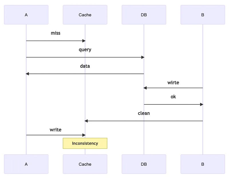
Even with this process, there are still problems, the most typical of which are the two problems mentioned in this article. The process of how stale sets occur is as follows.
Although B has cleared the cache, A is delayed for “some reason”, so the data in the cache is written to the old data, which is the data stale or inconsistent.
On the other hand, when a cache miss occurs in a highly concurrent system, then all these clients will query the database, in other words, the database will fall down in a short time due to high concurrency. This problem is also known as the Dogpile effect.
Facebook’s solution
How did Facebook solve these two problems? They use a lease mechanism, which is described in section 3.2.1 of the paper, but the explanation is not very complete, it is roughly the following two paragraphs.
A memcached instance gives a lease to a client to set data back into the cache when that client experiences a cache miss. Verification can fail if memcached has invalidated the lease token due to receiving a delete request for that item.
And.
We configure these servers to return a token only once every 10 seconds per key.
When writing data to the cache, it must carry the token that was obtained during the cache miss. The cache will first validate the token before updating, and if the token validation fails, then it will be ignored. The token will be cleared when the database is updated.
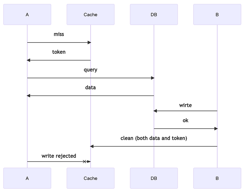
Let’s explain this with the sequence diagram.
The difference between this diagram and the problem one is the first interaction will get a token, when write cache need to carry the token, but because the token has been cleared after updating the database, so write cache will be rejected, this will solve the first problem.
As for the second problem is not difficult to deal with, just need to set the rules for the token release, every 10 seconds to send a token, if the client does not get the token then there is no authority to update the cache naturally there is no need to query the database, the Dogpile effect can be solved.
Simple implementation
To implement this logic is not so difficult, let’s use Python and Redis to write a simple example.
classCache: def__init__(self): # ignore implementation defget(self, k): v = self.redis.get(k) token = random.getrandbits(64) # Facebook says the token has to be 64 bit. ret = self.redis.set(f'{self.prefix}#{k}', token, 'NX', 'EX', 10) # 10s for token refresh return (v, token if ret == 'OK'elseNone) defset(self, k, v, token): saved_token = self.redis.get(f'{self.prefix}#{k}') if token == saved_token: ret = self.redis.set(k, v) else: ret = False return ret == 'OK'orFalse defclean(self, k): self.redis.del(k, f'{self.prefix}#{k}')
To make it easier to understand, here we only show the core implementation and do not use Lua or other pipeline optimization methods.
In get, two values are returned, one is the result of the cache and the other is the token, if the original token still exists and has not expired, which means there is a possibility of thundering herds, then the token is not returned, and if the client does not receive the token, then he should not query the database.
In set, in addition to the key and value to write, we also need to carry the token, when the validation of the token fails, we don’t update the cache and just end it so as to avoid stale sets.
Conclusion
Stale sets and thundering herds are pretty common problems when using caches, and there are many solutions for them. But when I actually wrote the program based on Facebook’s solution, I realized that it can be so simple, which made me a bit surprised that we were “overthinking” before.
I believe that the simpler the solution, the better, and I will use Facebook’s solution to deal with the problem at hand in the future. In fact, there are many more methods and optimizations for dealing with caching at scale in this paper, making it a very worthwhile study.
Exploring Three Viable Approaches to Optimize Database Resources
There are always times when the available space in the database is exhausted, and we need to take action.
Generally, the most common approach is vertical scaling, also known as scale-up, which involves increasing the specifications of the machine directly to expand the available space. Another alternative solution is horizontal scaling, also known as scale-out or sharding, which enhances overall available space by distributing data across different machines.
However, both scale-up and scale-out involve costs, and these can be substantial. For organizations with budget constraints, neither of these approaches may be immediately feasible. So, what can be done?
In such cases, the only option is to squeeze out as much space as possible from the existing machines, no matter what it takes, just pure squeezing.
In this article, we take MongoDB as an example to explore the viable approaches for squeezing out available space.
Remove useless index
Indexes are a trade-off of space for time to improve query performance. Therefore, if unused indexes can be identified and removed, the initially consumed space can be reclaimed.
Why do indexes become redundant?
There are several common reasons as follows:
Because MongoDB’s WiredTiger is a B-tree-based storage engine, it has a feature known as the leftmost-prefix. Thus, if a new index and an old index have the same prefix, the old index can be safely removed without affecting query performance.
Due to feature iterations, some queries that were required initially are no longer in use.
Regarding the first point, we can easily identify which indexes can be removed by carefully scanning each index. However, for the second point, some additional preparation is necessary.
We need to know which indexes are not being used. Apart from tracing clues from the code, there is a more efficient approach, which is to directly examine the index metrics. In the case of MongoDB, the $indexStatsaggregation operation can provide statistical data on the indexes.
By comparing the statistics from two time periods, we can determine which indexes are not being used.
Remove useless data
The above-mentioned approach of deleting indexes is a relatively straightforward solution that does not affect the production environment. However, if more available space needs to be squeezed out, consider deleting unused data.
Defining what constitutes unused data entirely depends on the application. For instance, some applications use flags to mark softly deleted documents, allowing these softly deleted documents to be removed or archived to cold storage.
Another scenario involves time-series data, where defining how old the data should be before it can be deleted becomes relevant. However, whichever solution is chosen depends entirely on the application.
Reshard
This is a more advanced approach compared to the previous two, directly impacting the performance of the production environment.
If the MongoDB cluster is already a sharded cluster but some collections have not been sharded, setting the appropriate shard key and enabling sharding can be a relatively straightforward process.
However, if all collections have already been sharded, it’s essential to examine which collections have uneven data distribution. Consider modifying the shard key and even taking further steps to rebalance. Phew, as of MongoDB 5.0, we can finally reshard a collection.
I previously wrote an article describing how to correctly design a shard key to achieve as even a data distribution as possible.
We can determine whether data distribution is uniform by using the command sh.status(). This command provides explicit information in the output regarding how many shards are being used for a collection and how many chunks each shard holds. A chunk represents the unit of data distribution.
However
It seems like we have several approaches that should all be effective if carefully implemented, right?
In reality, after implementing the second and third approaches, observing the available space reveals no improvement. In fact, it may even worsen, especially after executing the third approach.
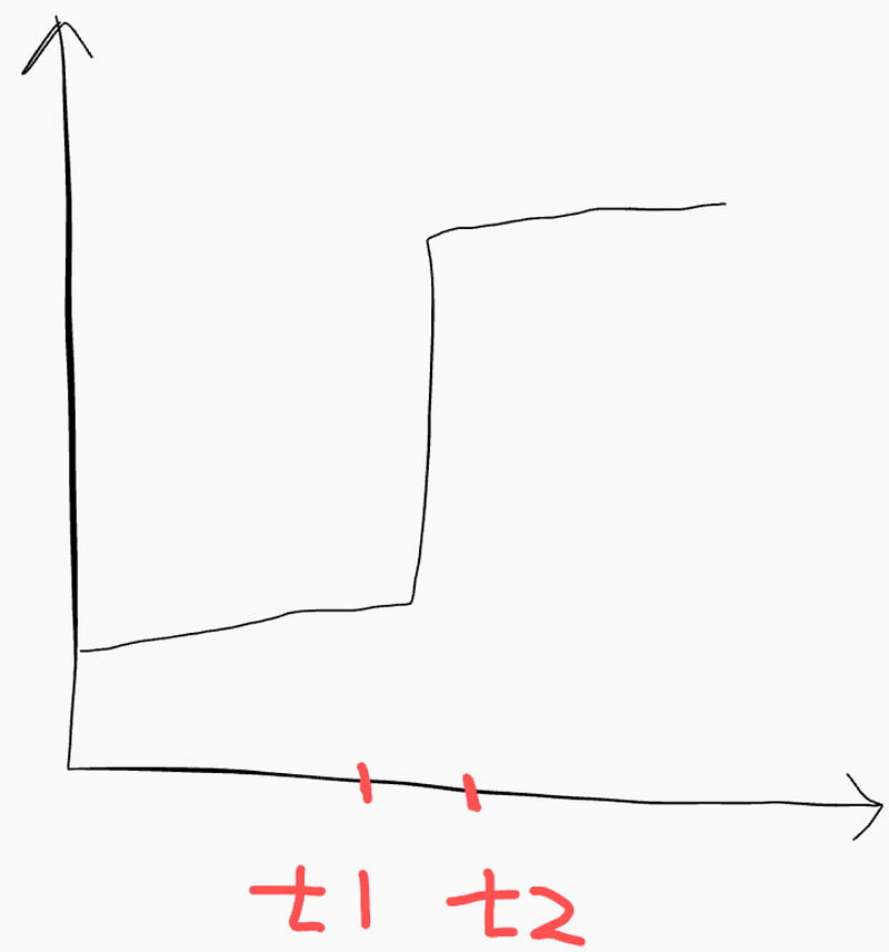
The following diagram illustrates the usage space of a particular shard on the y-axis over time on the x-axis. Here, t1 denotes the initiation of sharding, while t2 represents the completion of the sharding process.
We aimed to shard a collection that had not been sharded yet to release the available space in the original shard. However, as we can see from the diagram, after the sharding process was completed, the situation worsened, which was entirely contrary to our expectations.
Why did this happen?
The reason lies in WiredTiger’s behavior. After deleting documents, it does not immediately release the space. Instead, it retains the already allocated space, ensuring prepared chunks for future data writes in the collection.
This intention is well-meaning, as disk I/O performance is poor, and having a pre-arranged “clean slate” is valuable. However, this contradicts our goal of having the data disappear immediately after deletion. Hence, we see that although data is deleted, the available space does not increase.
Why did the diagram not only fail to decrease but also grow?
During the sharding process, to enable more efficient sharded queries, an index is created on the shard key. The additional space consumption represents the space occupied by these indexes.
Can we determine how much space WiredTiger has covertly consumed? The answer is yes.
Executing the commanddb.collection.stats() yields an output segment that describes “file bytes available for reuse,” representing the space that has been covertly taken.
If we can find it, we can certainly reclaim it. Running the compactcommand accomplishes this. It’s worth noting that the space regained through compact can only be used by the same collection, so the problem remains unresolved.
To enable all collections to reuse the occupied space, a complex procedure is required. Let me simplify the explanation.
When we add a new member to a ReplicaSet in MongoDB, the new member executes an Init Sync to synchronize the current data. However, this Init Sync only synchronizes actual data and not the occupied space. In other words, the new member does not occupy the available space.
Thus, if we gradually replace all the members in a ReplicaSet, we can obtain a new cluster (or Ship of Theseus) with the same dataset but without the occupied space. However, this process requires a “slight” additional budget to enable an extra machine as a new member, which is no longer necessary after the entire replacement process is complete, resulting in significant savings compared to scaling up or scaling out.
Conclusion
For any organization, finances are always a significant concern, particularly when it comes to database expenses, which can be quite substantial. While we aim to minimize costs wherever possible, the options available to us are limited. However, let’s quickly summarize the three methods to squeeze out available space:
Remove useless indexes
Remove useless data
Reshard
These three methods are in his order of precedence, with the first one being the quickest to implement and having the least impact on the production environment, and vice versa.
Moreover, executing solutions 2 and 3 requires additional processes to ensure that the space is genuinely available and not occupied.
Perhaps there are some secret techniques that I haven’t thought of yet. Feel free to share them with me.
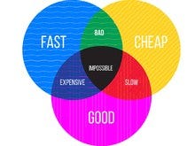
We can only have two of the three, and the price of being fast and good is expensive. Is there any way to do it as fast, as good and as cheap as possible? I believe the following article will be helpful.
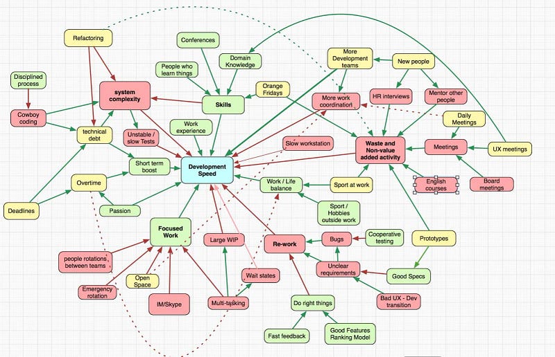
Apptio is an enterprise IT management solutions company with several programs for managing agile development processes. Acquired by IBM in June 2023, Apptio went from delivering a promising product to incubation and graduation in just a few years, itself a very agile company.
They wrote the above methodology on how to accelerate software development, and it’s a great read as it paints a detailed picture of the various software development scenarios.
Here’s a quick summary of some of the key points.
The blue blocks are our ultimate goal, to speed up development.
The red blocks are those that slow down development, and of course, the fewer the better.
The green blocks indicate items that will increase development speed, i.e. the more the better.
The yellow blocks mean that the right amount of these items will increase the speed, but too much will slow it down.
So, let’s look at the picture and tell the story.
We should:
Reduce system complexity
Reduce re-work
Focus on work
Reduce non-value added activities
Do refactoring properly
And so on.
But what exactly should be practiced? The article explains the details, so I won’t write it all out, I recommend to read the article carefully, I feel it is well worth reading!
Navigating the Path to Clean Code in Real-world Scenarios
How to design and implement clean architecture more easily has been described in detail in my previous articles. If you are interested in the details, you can refer to the following series of articles.
Instead of deeply diving into how to design and implement a clean architecture, this article will answer a question that we often encounter.
When should I consider clean architecture?
The main reason for asking this question is we often don’t design code with a clean architecture mindset from the start, but rather decide at some point to do a refactoring and introduce clean architecture.
This is a natural process because we don’t always have the ability to figure out how to encapsulate the domain in the first place, and we don’t always have the time to have a complete design at the beginning.
So, when should we refactor? And how? These two questions will be the core of this article.
Case Study
To answer these two questions we need a practical example, so let me describe my thought process using a chatbot.
Suppose I want to use a chatbot to implement an accounting program. The reason why I chose chatbot is to avoid complicated interface interactions, I just need to talk to my usual IM App to achieve the goal of accounting.
The overview of chatbot is as follows.
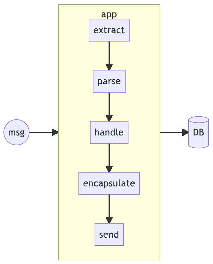
The user sends commands to the chatbot through a conversation, and the chatbot receives the message, encapsulates it and sends it to a web service via a webhook; the web service extracts the content with the corresponding SDK, processes the commands, and then sends the results back to the user. The process of processing the message involves accessing the database.
The code flow of the app is organized in the following five steps.
Extract: Use SDK to extract the received request.
Parse: Parses the message into a corresponding command.
Handle: Execute the command and generate the result. Interaction with the database also occurs at this stage.
Encapsulate: After handling the request, the result is packaged into the correct format by the SDK.
Send: Finally, the result is sent back to the user.
The whole core process will be the second and third steps. Without considering the clean architecture, the entire code would look like the following.
1
2
3
4
5
6
7
if msg == 'ooo': ret = user_guide() elif msg.count('x') > 10: ret = insert_items() elif'oxo'in msg: ret = get_report() # and so on
By parsing the msg, we know the command and take the corresponding action, in other words, this is the business logic of the whole program.
In the above example, we have three kinds of commands and three handlers, which correspond to the three common functions of a accounting program.
ask how to use the program.
write in accounts.
generate reports.
I believe that adding a fourth command would be too painful for some people, and I would start thinking about refactoring it at about this point.
So to answer the first question: when should I consider refactoring with clean architecture?
The answer is simple: when the requirements keep iterating and the code becomes difficult to maintain.
But how to refactor? How to introduce clean architecture?
Refactoring
According to the above description, we have two main business logics.
Parser
Handler
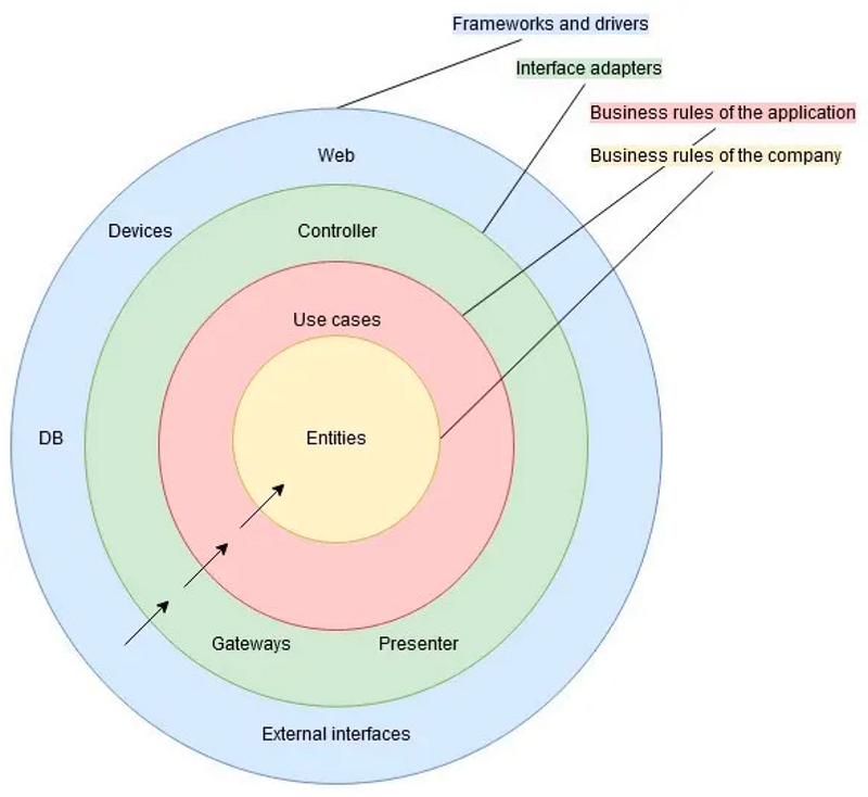
Let’s review the onion architecture one more time.
Calling chain has to go from the outside to the inside, and the most inside is business logic.
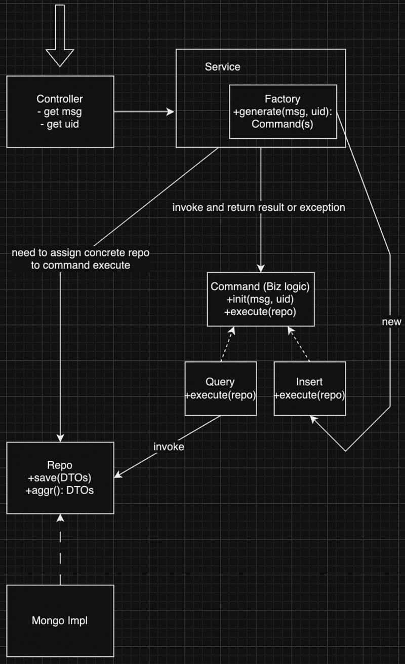
So I will plan the refactored components as shown below.
Let me explain these components.
Controller: Handles the in/out of the webhook and gets the actual message and user id of the caller with the SDK.
Service:
Call Factory to get concrete command.
Execute Command directly and get the result, may be a string or an exception.
Factory: Handles the logic of generating the Command, i.e. the command parser.
Command: Handles the actual business logic, i.e. the handler, and is responsible for converting the result of the repo to a string.
Repo: handles database calls and wrapping the database format into a DTO, no logic involved.
Splitting the domain in this way has several advantages.
Factory unit tests only need to have msg and match Command type, the implementation is quite simple.
Command encapsulates the full behavior of individual commands and isolates the database implementation, so unit testing can easily replace the database through dependency injection and just verify business logic.
Repo provides an interface to the database and wraps the format of the manipulated data into a DTO, providing a common specification.
Back to the onion architecture, Factory and Command are considered business logic, i.e., Entity, and Service is responsible for calling the Entity in order and doing the corresponding error handling, which belongs to the middle Use Case layer. The outer Controller handles the SDK and web framework, and calls the Service to get the result.
The only thing need to discuss is the outermost layer of DB, in the class diagram is actually Mongo Impl, through the implementation interface to make it out of the bottom layer of the calling chain, all the classes will only touch the Repo rather than the implementation of MongoDB. How to explain the source of the calling chain, i.e. the outer layer, is the DB?
The reason is that the outer layer of the code needs to prepare a concrete repo of the Mongo Impl and pass it to the Controller. In my current implementation, I’ve changed my approach a little bit by passing the class type instead of instance.
A similar implementation can be found in my previous Golang tutorial.
Then the “Command”, where the actual business logic is executed, and the following examples will only pick one of them as a demonstration.
1
2
3
4
5
6
7
8
9
10
11
12
classInsertManyCommand(Command): defexecute(self, repo_cls): tokens = [x.strip() for x in self.msg.split(',')] data = [] for token in tokens: item, cost = [t(s) for t,s inzip((str,int), token.split())] data.append(Item(item, cost)) repo = repo_cls(self.uid) success_cnt = repo.insert_many(data) returnf'Successfully wrote {success_cnt} record(s)'
Conclusion
Let’s go back to the title, when should we start considering clean architecture? I feel the answer is obvious, when we need to change the code but we don’t know where to start, that’s a good time to do it.
Why do I let my business logic consist of Factory and Command? Because once I’ve clarified the behavioral patterns of the bot, I can clearly recognize that two things are necessary: parsing and handling, so these two corresponding entities are created. In addition, when these two things are separated, the difficulty of unit testing is significantly reduced.
I can fully test parsing messages, and of course I can test every self-contained command completely.
When we mention clean architecture, will always make people think of hexagonal architecture or domain-driven development and other formal rules, but in practice to make the architecture clean, as long as the basic essentials will be enough, that is, the concept of the onion architecture.
Some of the design patterns used in this article, such as the factory method or strategy pattern. Even though I didn’t follow the textbook, I was able to achieve a good result.
When I drew that class diagram, I didn’t actually have a specific design pattern in mind, but rather, it was based on what shape I wanted the code to be organized into. I first thought about how I would like to decouple and individually test a command if I needed to add one, and then I created two components (Factory and Command) with this idea in mind.
Although Factory has a relatively simple role, I indeed thought for a while about what context Command would be responsible for. Take InsertManyCommand for example, there are these options.
The Service is responsible for tokenization and conversion to DTO.
The Repo is responsible for tokenization and writing directly to the database.
The Service handles the presentation of the result string.
All of these were eventually put into Command, because how the strings are split and how the results are presented should be part of the business logic, and naturally should be handled by Command, which is the core of the business logic.
Once we have a concrete idea, we can fill in the details of the class diagram, and then we just need to follow the diagram to write the program exactly as it is designed.
Lastly, my thoughts on ORMs. In fact, I don’t use ORMs to implement database access, but rather use pymongo with a custom DTO.
Why don’t I just use an ORM? The reason is that ORM will make developers overlook the existence of database and make clean architecture difficult to achieve.
From the onion architecture, we know the database is on the outer layer and should not be called by any object, but with ORM, we can easily develop the ORM as an entity into the inner layer of the onion architecture, and it even contains a lot of business logic. This is difficult to test and difficult to maintain, and is the worst situation of all.
Explaining Python 3.10’s new features with real-world examples
Pattern matching has finally been supported in Python since 3.10, and this feature, which is common to many functional programming languages, has been painlessly ported to Python.
However, for those of us who are new to pattern matching, it’s hard for us to figure out the right use cases and thus the code we write is not much different from an if-else, with at most a little more syntactic sugar in the if-else to allow for more fine-grained definitions of the variables.
To understand the real use case of pattern matching, we have to review the paragraph in PEP 635.
Much of the power of pattern matching comes from the nesting of subpatterns. That the success of a pattern match depends directly on the success of subpattern is thus a cornerstone of the design.
Nesting of subpatterns sounds a bit abstract, what are some practical examples of this property?
The easiest data structure to understand is the tree.
Taking a binary tree as an example, traversing from the top to the bottom, each node actually satisfies the following properties.
Each node will have an attribute of its own, as well as a child to the left and right, and this is the typical nested structure. Therefore, one of the most practical examples is to look for tree nodes that match the pattern.
AST Tree
AST tree is a very common method used for lint or syntax checking.
Suppose we have a requirement to check whether a source code has a direct call to print, then we can use if to compare the conditions and find out if the node that matches the condition violates the lint rule.
1 2 3 4 5 6 7 8 9
for node in ast.walk(tree): if ( isinstance(node, ast.Call) # It's a call and isinstance(node.func, ast.Name) # It directly invokes a name and node.func.id == 'print' # That name is `print` ): sys.exit(0) sys.exit(1)
From the above code we know we want to match a node ast.Call and it is a call function and the function name is print, three conditions in total.
Now, we know the pattern conditions we want to compare, let’s rewrite it as follows using pattern matching.
1 2 3 4 5 6 7
for node in ast.walk(tree): match node: # If it's a call to `print` case ast.Call(func=ast.Name(id='print')): sys.exit(0) sys.exit(1)
With pattern matching, we can make the conditions more straightforward by comparing them to the class definition we have in our head.
From the code we can see pattern matching makes comparing conditions simple, but that’s not the power of pattern matching, because we haven’t compared nested structures yet. Let’s look at the next example.
Parsing Tree
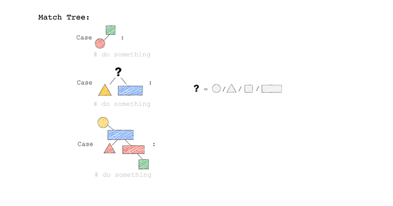
Suppose now I want to find some Patterns on a binary tree with various colors and shapes.
Given a tree of this kind, I want to know:
Is there a green square on the tree with a red circle attached to the left node?
Does the tree have any shape of any color, with a yellow triangle attached to the left node and a blue rectangle attached to the right node?
The tree has a yellow circle with a blue rectangle attached to the left node. For the blue rectangle, the left node is connected to a red triangle, and the right node is connected to a red rectangle. The red rectangle, the right node is connected to the green square.
Then our thinking model would look like the following diagram.
defFind(Tree): match Tree: case Square('green' , Circle('red') as left , _ ) as root: print(f'case1 \n {root = } \n {left = } \n ') case Geometric( _ , Triangle('yellow') as left, Rectangle('blue') as right, ): print(f'case2 \n {left = } \n {right = } \n') case Circle('yellow', _ , Rectangle('blue', Triangle('red'), Rectangle('red', _ , Square('green') ), ) as right ) as root: print(f'case3 \n {root = } \n {right = } \n ') case _: print('Not Found \n')
From this example, we can see the power of pattern matching, not only to compare nodes with explicit conditions, but also to compare fuzzy conditions as in case 2. It’s not just easier to write code, it’s easier to map the ideas we have in our head directly to the code.
In fact, database and big data engine optimizers make heavy use of pattern matching (not in Python) because the patterns that optimizers need to match are so complex that it would be very difficult to maintain code that simply uses if-else.
Conclusion
Pattern matching is a powerful technique, it’s not just a simple if-else or switch-case, it’s a “pattern matching”.
However, in our daily lives, we seldom really utilize the power of pattern matching, both because we seldom deal with a large number of nested structures, and because we misunderstand the scenarios applied to them.
Here’s a classic example from Stack Overflow. I’ve captured the answer with the most likes.
1 2 3 4 5 6 7
match a: case _ if a < 42: print('Less') case _ if a == 42: print('The answer') case _ if a > 42: print('Greater')
Is this really better than if-else?
1 2 3 4 5 6
if a < 42: print('Less') elif a == 42: print('The answer') elif a > 42: print('Greater')
I believe that most people don’t think so, and this is a typical misapplication scenario.
To sum up, the scenario where pattern matching is used is not conditional comparison, but pattern comparison. In addition, the real power of pattern matching is the nested structure.
Empower Sharding Strategy to Handle Cross-Shard Queries with Confidence
Before discussing sharding, let’s first talk about scaling. We all know that there are two types of scaling, one is vertical scaling, also known as scale-up, and the other is horizontal scaling, aka scale-out.
As for scaling, there are different ways for different purposes. For MongoDB, if we want to improve query performance, then vertical scaling is to improve the machine specs, while horizontal scaling is to increase the number of replicas so that the query can be executed on the idle replicas.
On the other hand, to increase the amount of data stored, for MongoDB, vertical scaling is still about improving the specs of the machine (in this case, the size of the hard drives), while horizontal scaling is about sharding, which is the main topic of this article.
Therefore, we have to understand that the purpose of sharding is to make the data evenly distributed so that MongoDB can store more data, not to improve the query performance. In other words, query performance will be improved by sharding as an extra, but not the main purpose.
Why specifically mention cross-shard queries in the title?
When we consider doing sharding, we will always consider carefully how to choose the shard key, choose the shard key and worry it will affect the production of the query performance, and consider rewrite all the query drastically. These concerns are actually unnecessary.
Let me conclude that if migrating to a sharded cluster from no sharding, as long as the shard key is chosen correctly, then it will only be better, not worse, because it’s a WORST case now.
Why so sure?
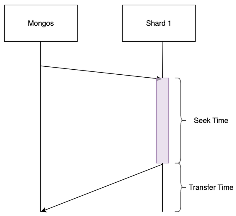
The formula for query time in database is as follows.
Ttotal = Ts + Tx
Ts is the retrieval time of the database itself, either by index or by scanning the full collection. Tx is the return time of the query result.
In addition, Ts and Tx have the following properties. Ts ∝ total data volume Tx ∝ result size
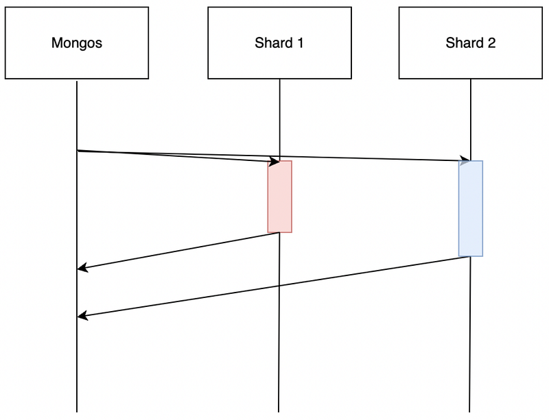
When we migrate this collection to a sharded cluster, then the above diagram will change a bit.
The formula will also change a little bit, but the principle is the same.
TclusteredTotal = Max( T1s + T1x , T2s + T2x )
Even if there is data skew happening, I believe we all agree the following conditions are true.
Tns < Ts
Tnx < Tx
Therefore, a conclusion can be deduced.
TclusteredTotal < Ttotal
Nevertheless, there are still some worst cases, for example, sharding is based on the data size rather than the frequency of data access, if there is busy collection(s) originally distributed in two shards without sharding, so they can consume all the resources of their respective machines individually. However, because of sharding, most of the data is distributed to the same shard, which competes for resources.
In other words, the precondition for the problem is the original MongoDB is nearly full and resources are almost exhausted.
How to choose shard key?
From the above introduction, we know as long as the shard key is chosen correctly, then we don’t need to worry about the performance of queries decreasing after sharding. Therefore, how to choose the shard key is pretty important.
I have already provided the ideal formula and described the details in my previous article.
Therefore, in this article, I will only outline which three types of bad cases must be avoided.
Low Cardinality
Suppose we choose an enum field as the shard key, and the range is fixed to [1, 2, 3].
Then even if we write 2 to the max, we still can’t start rebalance, and the maximum number of shards is 3.
Ascending
If we use a continuously incrementing field as the shard key, then we can ensure the chunks are evenly distributed, but it will continuously trigger a rebalance, and the performance will be horrible.
Furthermore, the data we need to query frequently is usually new, in other words, the query and the rebalance will often mix together, making the situation even worse.
Random or Hash Value
Another common choice is to use a random field (or hashing) as the shard key, which also ensures the chunks are evenly distributed and does not trigger frequent rebalances, but the rebalance overhead is increased.
MongoDB’s storage engine, WiredTiger, uses a storage distribution similar to MySQL’s InnoDB, i.e., the primary key (_id) is used as the storage unit (block), and similar primary keys are placed in the same block.
If we use random shard key, it will trigger random access instead of sequential access when we do rebalance.
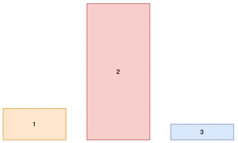
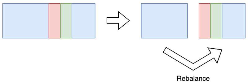
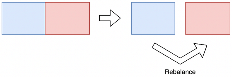
For instance, when a chunk is full and needs to be rebalanced, the data needs to be migrated across three blocks, and the entire rebalance time will be longer. This is far worse than the performance of a single block to complete the rebalance, as shown in the following diagram.
Conclusion
When we encounter a new problem, we often feel hesitant or even scared because it is unfamiliar.
What we need to do is to take a deep breath and return to the nature of the problem, analyze the core of the problem, and don’t be confused by the external appearance. Taking cross-shard queries as an example, when we use the database perspective instead of MongoDB to unpack the problem, the answer will be obvious.
Software engineering is already a stable field, most of the problems are similar in nature, so don’t panic, think carefully, most of the answers are not complicated.
For a public API to be called by a user, it is common practice to use versioning to control the impact. For example, when a user calls an API and expects certain results, a change in the API’s interface or behavior can cause unpredictable risks for the caller. Therefore, in practice, the original API will be tuned to version 1, and the modified API to version 2.
Users can be sure that calling the original version 1 API will not cause any problems, and the service providing the API can continue to iterate on the functionality, both sides of the development cycle can be independent of each other. Of course, maintaining two sets of APIs increases the maintenance effort for the service provider, so APIs have a lifecycle and don’t live forever.
In the case of the AWS services, the APIs called by the SDK have a version number (named by date), so it is recommended to specify the version of the used API in the production environment.
The following is an example of the AWS Python SDK, boto3, which according to the official document, api_versions should be specified in AWS configure. The version change of each service is available in this channel.
In fact, there are many different ways of implementing API versioning, and one interesting example is Shopify, according to Shopify’s official document, we know that Shopify releases one version per quarter and maintains only four versions at a time, i.e. one year.
Versions are date-named and embedded directly in the URL, and those out-of-date versions fallback to the oldest version in available support.
In other words, suppose the current four versions are as follows.
2023–07
2023–04
2023–01
2022–10
Then the call to 2022–07 would use the version 2022–10.
This is an interesting way of implementation, as the client has one year to make changes, and if it doesn’t, it will still work, but with unexpected results, instead of just crashing.
How to implement such a versioning mechanism? This article provides a possible approach.
Implementation approach
The full source is in the following repo.
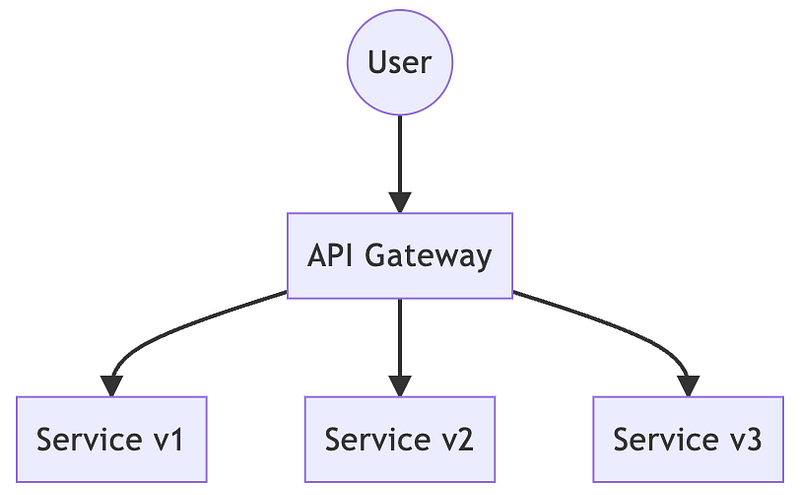
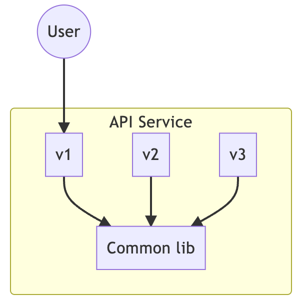
The overall implementation architecture is as follows.
All three services implement two URIs: /hello and /hi, which just print the URI with a version number.
For users, to call the corresponding service, they just put a prefix in front of the URI, e.g. curl http://localhost/v2/hello would print out
hello v2
In addition, calling a non-white-listed (v1, v2 and v3) version will fallback to v1, e.g., curl http://localhost/v4/hello will print
hello v1
The core of this experiment is nginx on the gateway.
If the location matches the previous 3 rules, then rewrite the original URI, remove the prefix and redirect to the corresponding service, if it doesn’t match the previous rules but matches the version specification (v plus integer), then redirect to the v1 service anyway.
By using nginx regex, we can make the version match the corresponding service and implement the extra fallback mechanism.
Conclusion
Actually, there is another approach to provide various versions of the API in the original service, for instance, opening several endpoints directly in the API service as follows.
/v1/hello
/v2/hello
/v3/hello
Creating three versions of the API directly instead of adding a prefix to the API through the gateway is not recommended. If you don’t physically isolate them, it adds a lot of development overhead, as in the following real-world example.
When we need to modify the behavior of the common lib, it will inevitably affect v1, which makes it difficult to iterate on the functionality, and also introduces risk to the user.
Therefore, isolation at the physical level is more controllable than isolation at the logical level. This article provides a possible approach, but there are many other implementations that can achieve the same result, so feel free to share them with me.
An Open Source, Flexible and Powerful Event Tracking System
SNOWPLOW is a platform for tracking events, i.e. collecting various user behavior events and analyzing them. Nowadays, there are many famous similar products like Google Analytics, Mixpanel, etc., but in the open source ecosystem, SNOWPLOW has a place.
Although there is a paid version of SNOWPLOW, I can’t figure out any reason not to use Mixpanel instead of SNOWPLOW since I have to pay for it, but there are a lot of advantages I can put forward for the open source version of SNOWPLOW.
For example, the architecture is simple and easy to integrate with existing infrastructure, and there are many flexible components that can be customized. Most importantly, there are a lot of SDKs available for various scenarios, e.g., Web, Mobile apps and even backend systems.
This article will not introduce the use case of SNOWPLOW, because it has been introduced in detail in the official document. Instead, this article will introduce the architecture of SNOWPLOW and provide a free playground.
Why emphasize on free?
In fact, in the official SNOWPLOW document there is a quick start environment for the terraform, but it is deployed on AWS or GCP and uses a lot of paid services. For a beta player, maybe we just want to experience what it can do, but don’t want to pay for it, at least I don’t, then a local free test environment is necessary.
Architecture Overview
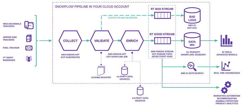
First of all, let’s take a quick look at the SNOWPLOW architecture.
There are three core components in the whole infrastructure, collector, enricher and schema registry, which are the fundamentals of SNOWPLOW. As for what kind of data warehouse or analysis engine to use, those can be freely matched and are not part of the SNOWPLOW package.
Collector: Collects events from the SDK, these events are raw data and therefore continue to be delivered to the enricher.
Schema Registry: The registry used in SNOWPLOW is a self-developed iglu, which is a service that manages JSON schema.
Enricher: After receiving the raw data, the first step is to validate it with the schema registered in the schema registry, and if it passes the validation, then it will be processed to produce a more analytical format and continue to send it to the next stage. As for the data to be sent to the data warehouse or Looker or other analysis platforms is based on demand.
One of the more interesting parts of the process is the enrichment stage, where here lists all the available plugins. Let’s take a practical example. An incoming event will only have an IP field, but subsequent analysis will depend on the geographic location, which can be enriched by the plugin IP Lookup.
This is a simple but powerful architecture that includes both validation and enrichment, and what’s more, the events are flexible in their format and can be customized to fit every need. In addition, these events can be downstreamed in a variety of ways based on demand, and can be flexibly integrated with the existing infrastructure.
This Github repository provides a docker-compose.yml, yes, we all love docker-compose. All the required components can be built locally and the usage is written in the README which should not cause any problems.
Also, for testing purposes, in addition to viewing the local database, I’ve put an additional Kafka management console at localhost:9021, which makes it possible to visually see each event.
All the settings of the components to be modified are located in the config.hocon under the corresponding folder.
Let’s describe the architecture of the test environment as follows.
There is a mock web with Javascript SDK installed, after entering http://localhost it will send some events to the collector periodically.
When the collector receives an event, it will store it in the database (atomic.events) and send it to Kafka.
When the Enricher receives an event, it first confirms the schema with the Iglu server, then performs basic enrichment and sends it to Kafka.
The final mock processor is to simulate how the enriched event should be handled.
The whole process is straightforward. After setting up the environment, we can observe the complete data flow in Kafka’s management console.
Conclusion
In fact, I have tried SNOWPLOW’s cloud-based Enterprise version, and the biggest difference I felt was the schema management. In the the open-source version, if we want to customize the event fields, we have to integrate Iglu’s REST API, and then we have to understand Iglu’s design concepts. However, in the cloud version, there is an easy-to-use UI that makes managing schema much easier.
Nevertheless, if we just want to do basic event tracking, I believe the open-source version of SNOWPLOW provides a good capability. Of course, if we want to use it more deeply, we need to understand and integrate it more comprehensively, which is also the price to pay for open source software.
In the previous article, we introduced three kinds of optimization mechanisms for Flink SQL as follows.
Reduce sub plan
Mini batch
Local-Global aggregation
These mechanisms correspond to some use cases individually. Among them, mini batch and Local-Global aggregation are both optimized for GROUP BY operations. However, in the previous article, we mentioned that even though both mechanisms can improve the performance of GROUP BY, they are not applicable to DISTINCT.
Therefore, in these articles, we will start by explaining the reason for this problem, and then we will introduce more optimization mechanisms.
Before explaining the problems encountered by DISTINCT, let’s review Local-Global aggregation with an example.
1 2 3
SELECT color, COUNT(DISTINCT id) FROM T GROUPBY color
This SQL command is a little different from the previous one, i.e., it uses DISTINCT, but it is similar to the previous one.
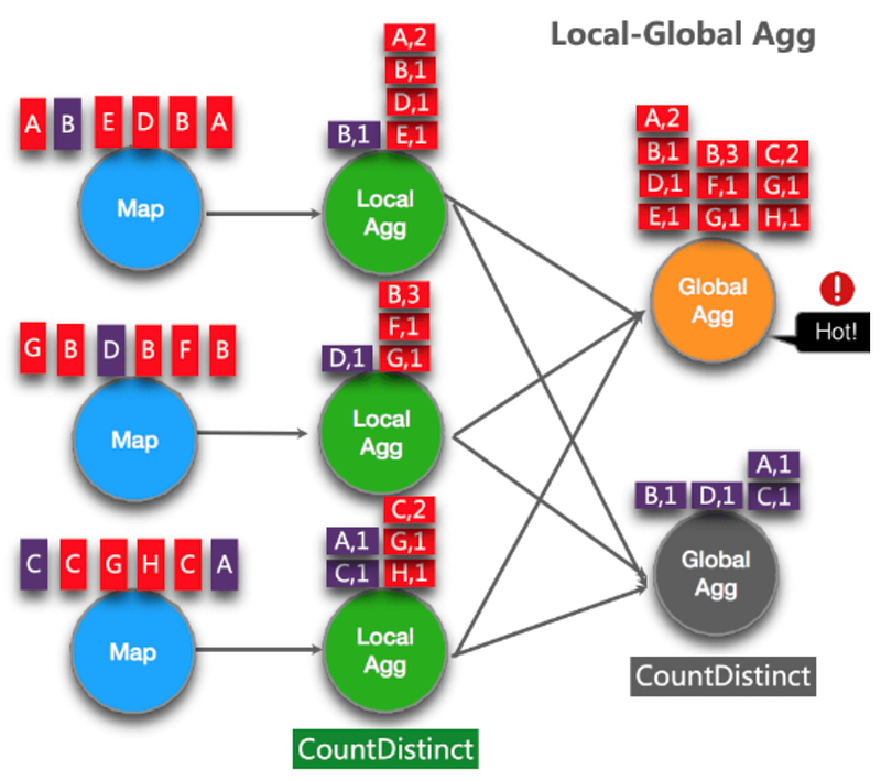
In Local-Global aggregation, we will do a first aggregation in the mini batch according to the color, and then we will do a second aggregation in the next operator with the results of the mini batch pre-aggregation.
As we can see above, even though we did the pre-aggregation in the mini batch, the effect is not significant because the operation DISTINCT is not able to merge. This also results in a lot of data in the final aggregation, and the data skew is not solved.
Since so, can we use id to group the data again during local aggregation? By splitting again, we can collect data with the same id together, and then we can merge them.
This is exactly the concept of Split Distinct aggregation.
Let’s use pseudocode to explain.
1 2 3 4 5 6 7
SELECT color, SUM(cnt) FROM ( SELECT color, COUNT(DISTINCT id) as cnt FROM T GROUPBY color, MOD(HASH_CODE(id), 4) ) GROUPBY color
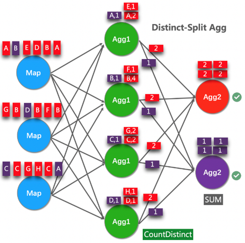
Split Distinct aggregation rewrites the original COUNT(DISTINCT id) into the above code. By first splitting the group with id, in this case into 4 groups, the pre-aggregation can be done.
Therefore, the actual operator will look like the following diagram.
We can see in the final aggregation stage that each operator needs to process the data more evenly, in other words, the data skew is solved.
There are two settings to enable Split Distinct aggregation.
table.optimizer.distinct-agg.split.enabled
table.optimizer.distinct-agg.split.bucket-num
The first setting is the feature toggle, and the second setting is the number of groups. Although we use COUNT as an example, any operation that is able to be merged can be split.
Nevertheless, one of the problems with Split Distinct aggregation is the significantly larger state and the increased state access. This is because the result of the split operation relies on the state to be persistent.
How to solve it?
Well, it’s as simple as a Local-Global aggregation after splitting the group. So the complete settings are as follows.
table.exec.mini-batch.enabled
table.exec.mini-batch.allow-latency
table.exec.mini-batch.size
table.optimizer.agg-phase-strategy: “TWO_PHASE”
table.optimizer.distinct-agg.split.enabled
table.optimizer.distinct-agg.split.bucket-num
We have turned on all the optimization settings related to GROUP BY. Be sure to remember that these come at a price, the most obvious of them is the increased use of computing resources.
JOIN Optimization
JOIN is a common practice for enrichment. In a normal SQL JOIN, it’s to find the same columns in the left and right tables and join the remaining columns together, but in streaming, it’s far from simple.
Because, there is no physical table in streaming.
So, in order to make the table concept, Flink will store the data in the state, and when there is an event input, the corresponding data can be taken out from the state immediately. However, there is a big problem with this approach, that is, the state will grow infinitely.
For example, suppose Flink has two streams, order and product. The order stream will keep append once there is a new order, and the product stream will have events for product creation, update and deletion.
Therefore, we write the following Flink SQL.
1 2 3
SELECT*FROM Orders INNERJOIN Product ON Orders.productId = Product.id
In the implementation behind Flink, all changes to the product are stored by the state, so that the corresponding result can be found as soon as the order event is generated, even if the product does not have any orders at all.
When there are a lot of products and the operator is running for a long time, this state can become very huge.
The most straightforward solution to reduce the unused state is to set TTL as follows.
table.exec.state.ttl
Nevertheless, when a product’s state is deleted, it can lead to unexpected results. In the above example, when the state of a product is deleted, if the order event of the same product comes in, the corresponding product information will not be found.
In addition to this simple and brutal approach, Flink also provides three alternatives to JOIN optimization.
It has a similar purpose to setting the TTL directly above, except that it allows the user to decide which field to use as the basis for time judgments.
1 2 3 4
SELECT* FROM Orders o, Shipments s WHERE o.id = s.order_id AND o.order_time BETWEEN s.ship_time -INTERVAL'4'HOURAND s.ship_time
Through this SQL, we can specify order_time and shipment_time as the basis of TTL, then Flink can know not to keep the state of the difference between order_time and shipment_time for more than 4 hours.
However, there is a limitation in this approach, in addition to the fact table on the left is append only, the dimension table on the right must also be append only, otherwise the time interval will be inconsistent.
Before we explain Temporal Join, let’s look at another example.
1 2 3
SELECT*FROM orders LEFTJOIN currency_rates ON orders.currency = currency_rates.currency
Assuming this is an international order, we need to know what the currency rate is for the order in order to calculate the sales performance of the product.
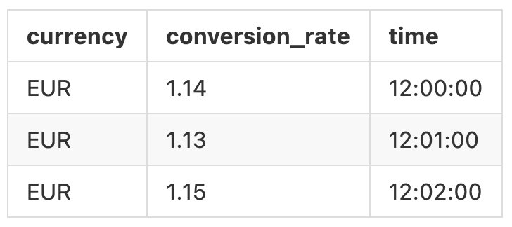
In order to keep the currency rates available at all times, Flink keeps a complete history of the currency rates. For example.
Therefore, the correct result can be obtained regardless of whether the order is placed at 12:00 or 12:01. However, we don’t really need this historical data, because we only need the current currency of the order, and the past history can be cleared out.
This is the concept of Temporal Join, only keep a latest mapping.
currency: conversion_rate
How to use this approach?
1 2 3
SELECT*FROM orders LEFTJOIN currency_rates FORSYSTEM_TIMEASOF orders.order_time ON orders.currency = currency_rates.currency;
One of the most special is FOR SYSTEM_TIME AS OF, this usage can be referred to SQL:2011 standard, this article will not dive into it.
The concept of Lookup Join is even more simple, since the state of Flink is so big and difficult to manage, it is better to go directly to the external data source, such as MySQL, for every event at the moment.
Time for space.
The entire syntax is written in the same way as the previous Temporal Join, using FOR SYSTEM_TIME AS OF, the only thing worth noting is the usage of proc_time.
1 2 3 4
SELECT o.order_id, o.total, c.country, c.zip FROM Orders AS o JOIN Customers FORSYSTEM_TIMEASOF o.proc_time AS c ON o.customer_id = c.id;
Because it is accessing external storage, Flink also provides some built-in optimization features.
In general, the process of accessing external storage is synchronous, sending a request and waiting for a response before moving on to the next one. However, Flink offers to send all requests at once and then wait for responses asynchronously, and it is turned on by default.
If we want to adjust it manually, we can refer to the Hints mentioned in the official document.
In addition, even if the external storage is accessed asynchronously, the actual operation will wait for the correct order of the responses after receiving them. If the order of the responses is not that important, then we can tell Flink not to wait for the responses to be in order.
Use the SQL command mentioned earlier as an example.
1 2 3 4 5
SELECT/*+ LOOKUP('table'='Customers', 'async'='true'. 'output-mode'='allow_unordered', 'capacity'='100', 'timeout'='180s') */ o.order_id, o.total, c.country, c.zip FROM Orders AS o JOIN Customers FORSYSTEM_TIMEASOF o.proc_time AS c ON o.customer_id = c.id;
It is most intuitive to tell the Flink optimizer what to do through Hints, so that it can be adjusted according to each command, but it is also possible to enable the global setting directly.
table.exec.async-lookup.output-mode
table.exec.async-lookup.buffer-capacity
table.exec.async-lookup.timeout
Mode and timeout are considered simple, as for capacity refers to how many IO command will trigger the actual JOIN operation. But I feel this is a bit abstract, set how much is appropriate is difficult to tell, it still needs to rely on experiments.
The last one is Window Join, which is similar to the concept of Interval Join mentioned earlier, and only retains a specific time range of states instead of all historical states. However, the window mechanism is very complicated and not required, so we will directly attach the example of the official document here without further explanation.
1 2 3 4 5 6 7 8 9 10 11 12 13 14
SELECT L.num as L_Num, L.id as L_Id, R.num as R_Num, R.id as R_Id, COALESCE(L.window_start, R.window_start) as window_start, COALESCE(L.window_end, R.window_end) as window_end FROM ( SELECT*FROMTABLE( TUMBLE(TABLE LeftTable, DESCRIPTOR(row_time), INTERVAL'5' MINUTES) ) ) L FULLJOIN ( SELECT*FROMTABLE( TUMBLE(TABLE RightTable, DESCRIPTOR(row_time), INTERVAL'5' MINUTES) ) ) R ON L.num = R.num AND L.window_start = R.window_start AND L.window_end = R.window_end;
To sum up, all kinds of JOIN rewriting are aimed at reducing the size of state.
The original JOIN will generate extremely large state, which will consume a lot of hardware resources if stored in memory, or generate a lot of hard disk IO if stored on persistent storage such as RocksDB, either of which will have a huge impact on performance.
Therefore, these four JOIN optimizations are all aimed at reducing the size of the state, but the exact solution to be used depends on the use case. The following is a brief list of the applicable scenarios.
Interval Join: Both the fact table and dimension table are append-only.
Temporal Join: Only the latest dimension is required.
Lookup Join: The dimension table is stored externally and does not care about dimension changes.
Window Join: Both fact and dimension tables have the window function enabled.
Conclusion
In the previous article, we introduced how to optimize general SQL commands and how to make GROUP BY more efficient. In this article, we introduced DISTINCT and JOIN.
I believe these two articles should have covered most of the Flink SQL scenarios, in fact, it is not hard to find that there are the following ways to make Flink SQL perform better.
Reducing invalid ( repeated ) commands
Reducing state access
Reducing the size of state
Reducing data skew
Every optimization has a proper scenario and a price to pay, and how to make Flink SQL perform better is a balance between these tradeoffs. Most of the optimizations are case-by-case and require understanding of Flink implementation before they can be applied.
These two articles are based on the latest stable version of Flink 1.17, maybe the URL of the attached reference will change, but I have explained the core concepts, so the new or old version of Flink should also be used as a reference.