Flink SQL Performance Tuning, Part 2
Flink SQL Performance Tuning, Part 2
Explaining the concept of Split Distinct aggregation and JOIN optimizations

In the previous article, we introduced three kinds of optimization mechanisms for Flink SQL as follows.
- Reduce sub plan
- Mini batch
- Local-Global aggregation
These mechanisms correspond to some use cases individually. Among them, mini batch and Local-Global aggregation are both optimized for GROUP BY operations. However, in the previous article, we mentioned that even though both mechanisms can improve the performance of GROUP BY, they are not applicable to DISTINCT.
Therefore, in these articles, we will start by explaining the reason for this problem, and then we will introduce more optimization mechanisms.
Split Distinct Aggregation
Before explaining the problems encountered by DISTINCT, let’s review Local-Global aggregation with an example.
1 | SELECT color, COUNT(DISTINCT id) |
This SQL command is a little different from the previous one, i.e., it uses DISTINCT, but it is similar to the previous one.
In Local-Global aggregation, we will do a first aggregation in the mini batch according to the color, and then we will do a second aggregation in the next operator with the results of the mini batch pre-aggregation.
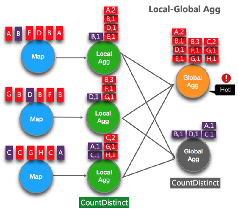
As we can see above, even though we did the pre-aggregation in the mini batch, the effect is not significant because the operation DISTINCT is not able to merge. This also results in a lot of data in the final aggregation, and the data skew is not solved.
Since so, can we use id to group the data again during local aggregation? By splitting again, we can collect data with the same id together, and then we can merge them.
This is exactly the concept of Split Distinct aggregation.
Let’s use pseudocode to explain.
1 | SELECT color, SUM(cnt) |
Split Distinct aggregation rewrites the original COUNT(DISTINCT id) into the above code. By first splitting the group with id, in this case into 4 groups, the pre-aggregation can be done.
Therefore, the actual operator will look like the following diagram.
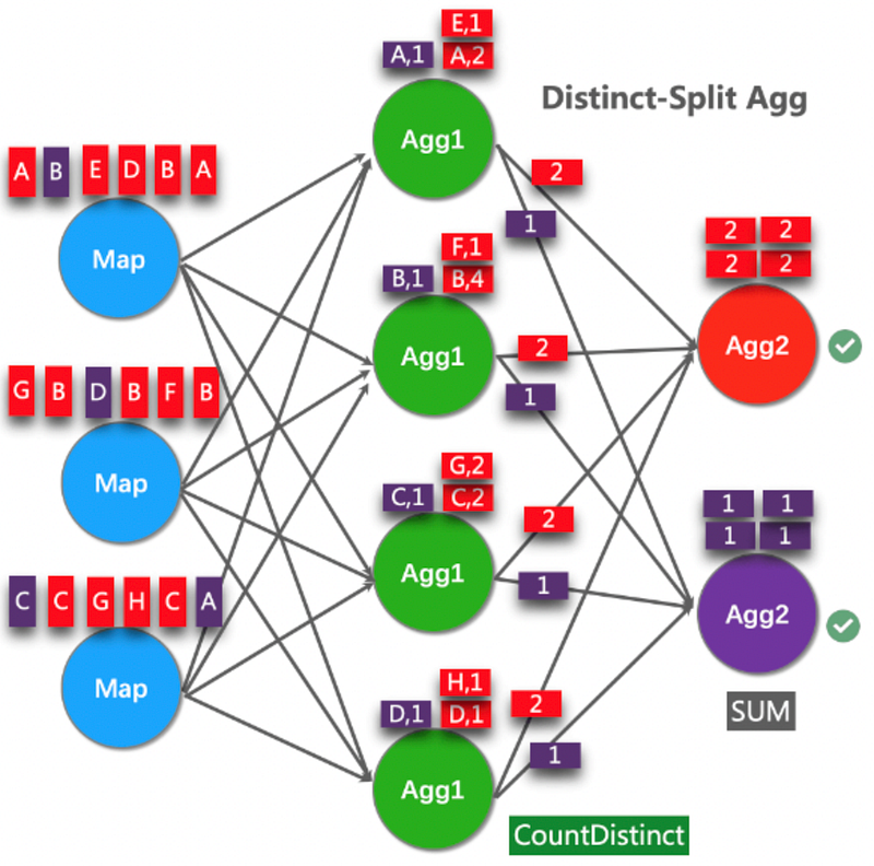
We can see in the final aggregation stage that each operator needs to process the data more evenly, in other words, the data skew is solved.
There are two settings to enable Split Distinct aggregation.
- table.optimizer.distinct-agg.split.enabled
- table.optimizer.distinct-agg.split.bucket-num
The first setting is the feature toggle, and the second setting is the number of groups. Although we use COUNT as an example, any operation that is able to be merged can be split.
Nevertheless, one of the problems with Split Distinct aggregation is the significantly larger state and the increased state access. This is because the result of the split operation relies on the state to be persistent.
How to solve it?
Well, it’s as simple as a Local-Global aggregation after splitting the group. So the complete settings are as follows.
- table.exec.mini-batch.enabled
- table.exec.mini-batch.allow-latency
- table.exec.mini-batch.size
- table.optimizer.agg-phase-strategy: “TWO_PHASE”
- table.optimizer.distinct-agg.split.enabled
- table.optimizer.distinct-agg.split.bucket-num
We have turned on all the optimization settings related to GROUP BY. Be sure to remember that these come at a price, the most obvious of them is the increased use of computing resources.
JOIN Optimization
JOIN is a common practice for enrichment. In a normal SQL JOIN, it’s to find the same columns in the left and right tables and join the remaining columns together, but in streaming, it’s far from simple.
Because, there is no physical table in streaming.
So, in order to make the table concept, Flink will store the data in the state, and when there is an event input, the corresponding data can be taken out from the state immediately. However, there is a big problem with this approach, that is, the state will grow infinitely.
For example, suppose Flink has two streams, order and product. The order stream will keep append once there is a new order, and the product stream will have events for product creation, update and deletion.
Therefore, we write the following Flink SQL.
1 | SELECT * FROM Orders |
In the implementation behind Flink, all changes to the product are stored by the state, so that the corresponding result can be found as soon as the order event is generated, even if the product does not have any orders at all.
When there are a lot of products and the operator is running for a long time, this state can become very huge.
The most straightforward solution to reduce the unused state is to set TTL as follows.
- table.exec.state.ttl
Nevertheless, when a product’s state is deleted, it can lead to unexpected results. In the above example, when the state of a product is deleted, if the order event of the same product comes in, the corresponding product information will not be found.
In addition to this simple and brutal approach, Flink also provides three alternatives to JOIN optimization.
It has a similar purpose to setting the TTL directly above, except that it allows the user to decide which field to use as the basis for time judgments.
1 | SELECT * |
Through this SQL, we can specify order_time and shipment_time as the basis of TTL, then Flink can know not to keep the state of the difference between order_time and shipment_time for more than 4 hours.
However, there is a limitation in this approach, in addition to the fact table on the left is append only, the dimension table on the right must also be append only, otherwise the time interval will be inconsistent.
Before we explain Temporal Join, let’s look at another example.
1 | SELECT * FROM orders |
Assuming this is an international order, we need to know what the currency rate is for the order in order to calculate the sales performance of the product.
In order to keep the currency rates available at all times, Flink keeps a complete history of the currency rates. For example.
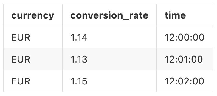
Therefore, the correct result can be obtained regardless of whether the order is placed at 12:00 or 12:01. However, we don’t really need this historical data, because we only need the current currency of the order, and the past history can be cleared out.
This is the concept of Temporal Join, only keep a latest mapping.
currency: conversion_rate
How to use this approach?
1 | SELECT * FROM orders |
One of the most special is FOR SYSTEM_TIME AS OF, this usage can be referred to SQL:2011 standard, this article will not dive into it.
The concept of Lookup Join is even more simple, since the state of Flink is so big and difficult to manage, it is better to go directly to the external data source, such as MySQL, for every event at the moment.
Time for space.
The entire syntax is written in the same way as the previous Temporal Join, using FOR SYSTEM_TIME AS OF, the only thing worth noting is the usage of proc_time.
1 | SELECT o.order_id, o.total, c.country, c.zip |
Because it is accessing external storage, Flink also provides some built-in optimization features.
In general, the process of accessing external storage is synchronous, sending a request and waiting for a response before moving on to the next one. However, Flink offers to send all requests at once and then wait for responses asynchronously, and it is turned on by default.
If we want to adjust it manually, we can refer to the Hints mentioned in the official document.
In addition, even if the external storage is accessed asynchronously, the actual operation will wait for the correct order of the responses after receiving them. If the order of the responses is not that important, then we can tell Flink not to wait for the responses to be in order.
Use the SQL command mentioned earlier as an example.
1 | SELECT /*+ LOOKUP('table'='Customers', 'async'='true'. 'output-mode'='allow_unordered', 'capacity'='100', 'timeout'='180s') */ |
It is most intuitive to tell the Flink optimizer what to do through Hints, so that it can be adjusted according to each command, but it is also possible to enable the global setting directly.
- table.exec.async-lookup.output-mode
- table.exec.async-lookup.buffer-capacity
- table.exec.async-lookup.timeout
Mode and timeout are considered simple, as for capacity refers to how many IO command will trigger the actual JOIN operation. But I feel this is a bit abstract, set how much is appropriate is difficult to tell, it still needs to rely on experiments.
The last one is Window Join, which is similar to the concept of Interval Join mentioned earlier, and only retains a specific time range of states instead of all historical states. However, the window mechanism is very complicated and not required, so we will directly attach the example of the official document here without further explanation.
1 | SELECT L.num as L_Num, L.id as L_Id, R.num as R_Num, R.id as R_Id, |
To sum up, all kinds of JOIN rewriting are aimed at reducing the size of state.
The original JOIN will generate extremely large state, which will consume a lot of hardware resources if stored in memory, or generate a lot of hard disk IO if stored on persistent storage such as RocksDB, either of which will have a huge impact on performance.
Therefore, these four JOIN optimizations are all aimed at reducing the size of the state, but the exact solution to be used depends on the use case. The following is a brief list of the applicable scenarios.
- Interval Join: Both the fact table and dimension table are append-only.
- Temporal Join: Only the latest dimension is required.
- Lookup Join: The dimension table is stored externally and does not care about dimension changes.
- Window Join: Both fact and dimension tables have the window function enabled.
Conclusion
In the previous article, we introduced how to optimize general SQL commands and how to make GROUP BY more efficient. In this article, we introduced DISTINCT and JOIN.
I believe these two articles should have covered most of the Flink SQL scenarios, in fact, it is not hard to find that there are the following ways to make Flink SQL perform better.
- Reducing invalid ( repeated ) commands
- Reducing state access
- Reducing the size of state
- Reducing data skew
Every optimization has a proper scenario and a price to pay, and how to make Flink SQL perform better is a balance between these tradeoffs. Most of the optimizations are case-by-case and require understanding of Flink implementation before they can be applied.
These two articles are based on the latest stable version of Flink 1.17, maybe the URL of the attached reference will change, but I have explained the core concepts, so the new or old version of Flink should also be used as a reference.
Originally published on Medium