Flink SQL Performance Tuning, Part 1

Posted on 2023-06-26 In Architecture Views:

Flink SQL Performance Tuning, Part 1

Explaining the concept of reduce sub plan, mini batch and Local-Global aggregation

Before talking about the tuning, we have to understand how Flink SQL works. In general, there are several steps as follows.

After receiving a SQL command, it is first parsed into a logical plan, and then the execution plan is generated by the optimizer. With the execution plan, the actual code for execution can be generated and finally turned into a job.

The only step we can control on the whole process is the optimizer.

And, the following are factors affecting Optimizer.

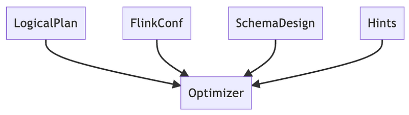
LogicalPlan: Generated from SQL parser, it can be said that a good writing style basically solves most of the performance problems.
FlinkConf: In Flink, there are many optimizer-related settings that can be adjusted.
SchemaDesign: Of course, the schema design also determines some of the performance, such as the primary key.
Hints: Although the optimizer will try to cover as many scenarios as possible, sometimes we still need to “tell” the optimizer what to do, and that can be done through hints.

Thus, this article will introduce a few common scenarios on how to tune.

Reuse Sub Plan

In Flink’s settings, table.optimizer.reuse-sub-plan-enabled is turned on by default. The functionality of this setting can be explained by a simple example.

1 2	INSERT INTO sink1 SELECT * FROM table WHERE a > 0; INSERT INTO sink2 SELECT * FROM table WHERE a > 0 AND b < 0;

First, convert the above two SQL commands into a logical plan.

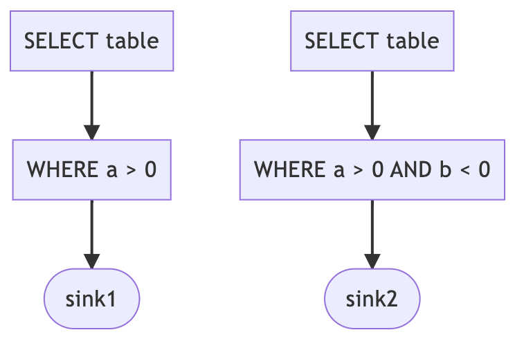
Then, after the reuse-sub-plan of the optimizer, the following execution plan will be generated.

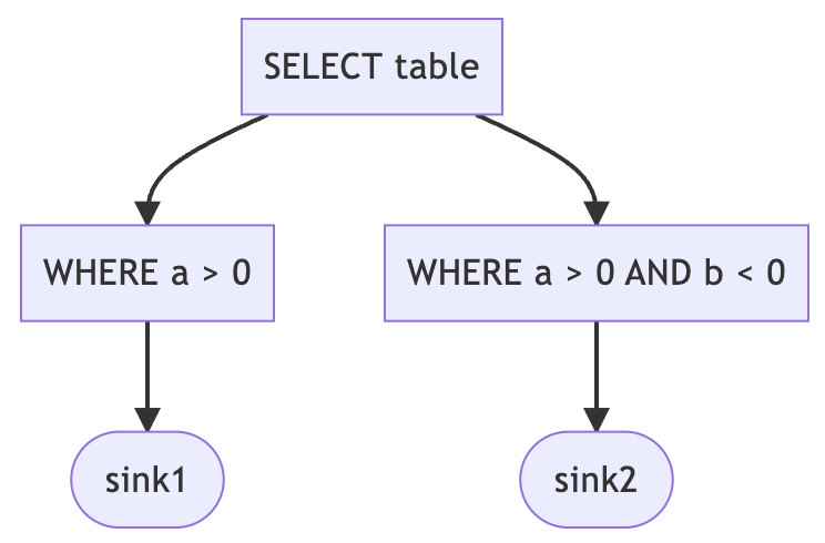
What the optimizer does is to merge the same parts, so that there is no need to repeat the process. But from our naked eyes, we can still see one identical part can be merged.

WHERE a > 0

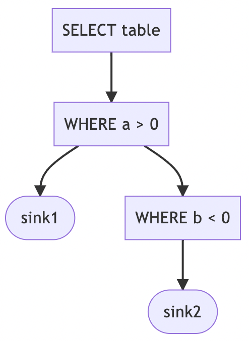
However, the optimizer does not recognize this clause, so we need to rewrite the original SQL to make the optimizer understand the merging rules for this filter.

1
2
3

CREATE TEMPORARY VIEW v SELECT * FROM table WHERE a > 0;  
INSERT INTO sink1 SELECT * FROM v;  
INSERT INTO sink2 SELECT * FROM v WHERE b < 0;

By creating a temporary view, the optimizer can generate a more efficient execution plan.

MiniBatch Aggregation

Mini batch is a built-in performance optimization mechanism for Flink. The mechanism behind is explained in the official document.

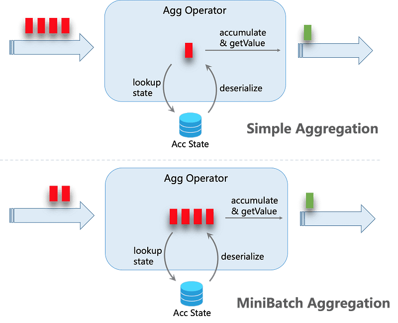
The above diagram shows an overview of a mini batch, in plain English, mini batch drastically reduces the number of accesses to the state.

Let’s use a practical example to explain this.

1
2
3

SELECT color, SUM(id)  
FROM T  
GROUP BY color

This is a typical SQL aggregation operation, in fact, the internal operation of Flink is each event must access the state once, so it can be summed up.

It is written in Python as pseudocode as follows.

def process(input):  
    color, id = extract(input)  
    ret = state.get(color)  
    ret += id  
    state.update(color, ret)  
    yield ret

When inputting an event, first of all we find its color, then we take out the previous summation result, then we add the id to it, and finally we write the result back to the state. The next event comes in and repeats the process.

Such a iteration will be extremely frequent to access the state, resulting in performance impact. So mini batch collects events and accesses the state only once for each specific color.

def mini_batch_process(batch):  
    for color in batch:  
        ret = state.get(color)  
        for id in batch[color]:  
            ret += id  
        state.update(color, ret)  
        yield ret

As you can see from the code above, the process of mini batch is to collect the events of the same color, so the sum of the same color can be done at once, without the need to access the state frequently.

To enable mini batch is as simple as turning on the settings of the optimizer.

table.exec.mini-batch.enabled
table.exec.mini-batch.allow-latency
table.exec.mini-batch.size

The first setting is on/off, the rest is to determine the size of the batch, which can be based on the amount or duration.

Local-Global Aggregation

There is a further optimization approach to GROUP BY, called Local-Global aggregation, which is an extension of mini batch.

The biggest problem of mini batch is that it will be grouped by color. If a particular color is especially large, then the downstream operator assigned to this color will have to process much more data, which is also called data skew. Therefore, Flink provides a mechanism to perform pre-aggregation in the mini batch in order to reduce the downstream load.

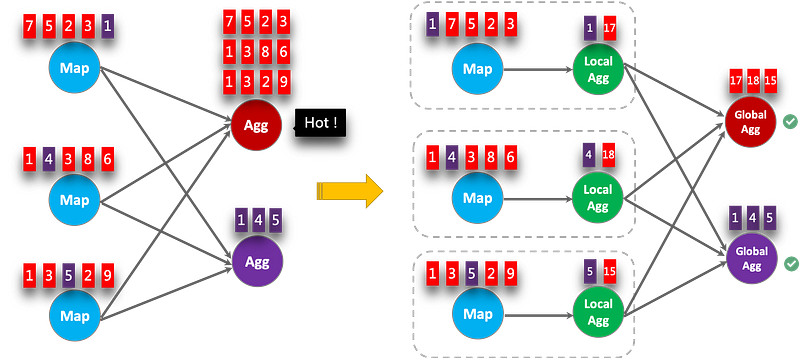
From the above diagram, we can see that after turning on Local-Global aggregation, the summation operation will be done inside the mini batch, and the last data aggregation will be done with a small amount of data. In the example red Agg, the amount of processed data will be changed from 12 to 3, i.e., the data skewing problem is solved.

To enable Local-Global aggregation, it is necessary to use the following settings in addition to the mini batch already enabled.

table.optimizer.agg-phase-strategy: “TWO_PHASE”

Conclusion

This article first introduces three of Flink’s built-in optimization mechanisms:

Reduce sub plan
MiniBatch aggregation
Local-Global aggregation

Only the first one is enabled by default, but there is still room for manual optimization. The other two are turned off by default, especially the Local-Global aggregation, which requires an additional mini batch to be enabled in addition to the two phases.

Since these mechanisms look so good, why are they not turned on by default?

Because, these mechanisms are not without cost.

In the case of mini batch, when mini batch is turned on, it means the freshness of data will be affected, depending on the mini batch settings.

In addition, Local-Global aggregation is not available for all operations. It is only used for aggregations that can be merged, such as SUM, MAX, COUNT, etc., and not for DISTINCT. Moreover, Local-Global aggregation increases the computation complexity and therefore consumes additional computing resources, which is not always reasonable if the data skew is not large.

These optimization mechanisms must be understood before using in order to use them correctly, and turning them all on unconditionally may lead to counterproductive results.

Of course, Flink’s optimization mechanism is not just these, next time we will talk about DISTINCT and JOIN which are not covered in this article.

Originally published on Medium