CT Wu

A Proven Theory of the Architect’s Difficulties

As an experienced architect, I have interviewed many candidates. But I have always had one question in my mind: why is it so hard to find candidates who meet the expectations?

Recently, after reading a study, I was able to answer this question in a more systematic way. The topic of this study is: Talent vs Luck: the role of randomness in success and failure.

It is also the 2022 Ig Informal Lecture for the Economics Prize.

Before we explain the connection between the architect’s difficulty in finding and this study, let’s quickly summarise the study.

To make a long story short, a person’s success has nothing to do with talent, but only with luck. To put it further, “Success is 1% genius and 99% luck”.

However, Thomas Edison told us that genius is 1% inspiration and 99% perspiration. In other words, to be successful, effort is only 0.99%.

Why are so few candidates qualified to be architects?

Because being an architect is not something you can do just by working hard, it’s very much a matter of chance.

Wait, that’s a bit arbitrary, isn’t it?

In fact, every single one of those interviewed was a good senior engineer — yes, every single one.

They all excel in their positions and have a good grasp of what they are responsible for. Even a team leader or manager who hadn’t actually written code in a long time still had a deep understanding of the service they were working on.

However, these candidates were eliminated.

The reason was simple: not enough experience. Yes, I agree that they can all fully handle one or a few microservices. But the volume of these microservices was just not there, either because they lacked the volume of traffic and high-frequency reads and writes, or because they lacked the complexity and interaction with other systems.

This kind of experience is no match for an architect of a high-volume e-commerce platform.

Did you notice a key point? They all do their jobs well or even brilliantly, but they are still inexperienced.

Specialist vs. Generalist

This is actually the difference between I-shaped talents and T-shaped talents, i.e. Specialist and Generalist.

If you want to become a qualified architect, it is not enough just to do a good job. But to be honest, even if you work very hard, you may not be qualified. As I mentioned at the beginning, whether you can become an architect or not is mostly a matter of luck.

• If you are lucky enough to have worked for a large enterprise, then there is a little more possibility.
• If, luckily, the company is willing to invest in various training, then there are more possibilities.
• If you are lucky enough to have friendships with architects, then you have a little more possibilities.

Can’t we learn the skills we should have by our own efforts?

Yes, but it’s really hard.

If you don’t see how wide the world is, you can’t imagine what you need to learn.

There is a Chinese idiom, “Frog in the bottom of a well”. A frog who lives in a well all his life cannot know the outside world.

Back to the architect’s perspective, let’s look at a few real-world examples.

How do you know you need to learn caching if a system works well with one database and one API service?

How do you know you need to learn sharding if the amount of data can always be carried by a single database?

How do you know you need to learn message queuing if the logic of the system is simple and can be responded in a short time?

More specifically, if a system does not have any search requirement, how do you know you need to learn Elasticsearch?

All these are the vision that an architect needs to have, so do you know why most of the time you need to rely on “luck”?

Even so

There are still possibilities for us to try our best.

• Read more books.
• Attend more seminars.
• Visit more blogs.

Even if we don’t know what’s missing, we can still become what we want to be by learning through various channels.

Architects are on a never-ending journey of learning.

Conclusion

We’ve talked a lot about what it takes to be an architect, and explained why it’s so hard to find a qualified candidate, but I have to say that being an architect is just one of the “choices” in a career.

It doesn’t mean an architect is superior, it doesn’t mean an architect is invincible, and it doesn’t mean an architect is better than a senior engineer.

If learning is your hobby, then architect is a good choice.

But a senior software developer is also a good choice.

Originally published on Medium

Netflix的首頁是經過客製化的，會根據使用者的喜好有不同的外觀，當然，推薦影片的種類也會完全根據使用者的偏好。要做到這種程度，是因為在系統背後有一個應用程式會根據各種演算法將好的UX遞送給使用者。

這個應用程式稱為RMI (Real-time Merched Impression)，其架構如下。

graph TD
    imp[Impression Source] --> kb1[KeyBy] --> join[Join] --> rmi[RMI Sink]
    pb[Playback Source] --> kb2[KeyBy] --> join

Generating Avro Schemas from Go types

To implement auto data ingest, reflect go struct into Avro

Previously, I have introduced the evolutionary history of data infrastructure, and I have also introduced real-time data analysis in detail.

• Evolutionary Data Infrastructure
• The Infrastructure Stack for Real-Time Data Analysis

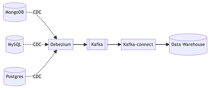
Both of these articles mention a key player, Debezium. In fact, Debezium has had a place in the modern infrastructure. Let’s use a diagram to understand why.

This architecture diagram should be consistent with the data ingest path of most data infrastructures. In order to store and analyze data in a unified way, centralizing the data in a data warehouse is a general solution.

Debezium captures data changes from various source databases and then writes them to the data warehouse via Kafka and Kafka’s consumers. In other words, Debezium is also a Kafka producer.

This architecture looks fine, once there are changes in the data will be captured by Debezium and eventually written to the data warehouse, but there is actually a difficult problem behind needs to be solved, that is, the database schema. In order to provide data analytics, the data warehouse is “schemaful”, but how to make the schema of the data warehouse align with the schema of each source database?

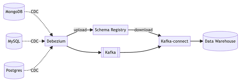
The good news is Debezium supports schema registry, it can capture DDL changes from source databases and synchronize them to the schema registry so that Kafka consumers can get schema from the schema registry and synchronize the schema in the data warehouse.

Let’s make the architecture mentioned above even more complete.

The most common format for describing schema in this scenario is Apache Avro.

Unfortunately, a schemaless database like MongoDB doesn’t have DDL at all, so of course Debezium can’t capture DDL, then how does Debezium upload the schema in this scenario? The answer is to guess, by getting the data to determine the data type, and write the type into the schema registry.

As you can imagine, this is very risky, and the data warehouse schema often faces compatibility challenges due to such guessing. Therefore, there needs to be a way to proactively upload the schema so that the Kafka consumer can correctly recognize the data type and correct the schema of the data warehouse.

Knowing it intellectually is one thing, but knowing it emotionally is quite another.

The story is this: our microservice is developed in Golang and uses mgm as the ORM for MongoDB.

In Golang, we use struct as a Data Transfer Object (DTO), and in the mgm scenario, these DTOs can be marshaled as JSON. So, what we need to do is to generate the corresponding Avro schema based on the definition of struct.

Therefore, I made the following go module.

The use of this go module is quite simple.

If we have a struct as follows.

1
2
3
4
5
6
7

type Entity struct {  
	AStrField    string  `json:"a_str_field"`  
	AIntField    int     `json:"a_int_field"`  
	ABoolField   bool    `json:"a_bool_field"`  
	AFloatField  float32 `json:"a_float_field"`  
	ADoubleField float64 `json:"a_double_field"`  
}

Then just import the module to generate the corresponding Avro.

1
2
3

import "github.com/wirelessr/avroschema"  
  
avroschema.Reflect(&Entity{})

The result will be an Avro JSON.

1
2
3
4
5
6
7
8
9
10
11

{  
    "name": "Entity",  
    "type": "record",  
    "fields": [  
      {"name": "a_str_field", "type": "string"},  
      {"name": "a_int_field", "type": "int"},  
      {"name": "a_bool_field", "type": "boolean"},  
      {"name": "a_float_field", "type": "float"},  
      {"name": "a_double_field", "type": "double"}  
    ]  
}

In addition, the module also supports various complex types and nested types as follows.

• array and slice
• map
• struct in struct
• time.Time
• array of struct
• etc.

Of course, the omitempty tag used by JSON in Golang is also supported.

Fields marked with omitempty become Avro’s union type, which is an optional field. Let’s take a more complicated example.

1
2
3

type Entity struct {  
	UnionArrayField []int `json:"union_array_field,omitempty"`  
}

If it is an optional int array, then it will become a union type with null when converted to Avro.

1
2
3
4
5
6
7
8
9

{  
    "name": "Entity",  
    "type": "record",  
    "fields": [  
      {"name": "union_array_field", "type": ["null", {  
        "type": "array", "items": "int"  
      }]}  
    ]  
}

More detailed tests can be found in the unit test file: reflect_test.go.

However, this is not enough for us, because we need to support various special types in mgm, such as primitive.DateTime or primitive.ObjectID, and most especially mgm.DefaultModel.

Therefore, it is necessary for this module to provide customization capabilities to extend support for more special types, thus, a plugin is provided for this module to be used. To support mgm, you can use the already made submodule.

The following is an example of a struct that uses the mgm type.

1
2
3
4
5
6
7
8
9

type Book struct {  
	mgm.DefaultModel `bson:",inline"`  
	Name             string             `json:"name" bson:"name"`  
	Pages            int                `json:"pages" bson:"pages"`  
	ObjId            primitive.ObjectID `json:"obj_id" bson:"obj_id"`  
	ArrivedAt        primitive.DateTime `json:"arrived_at" bson:"arrived_at"`  
	RefData          bson.M             `json:"ref_data" bson:"ref_data"`  
	Author           []string           `json:"author" bson:"author"`  
}

To support these special types, you can use the built-in custom MgmExtension. This works just like the original Reflect, except it requires the use of a customized instance.

1
2
3
4
5
6
7
8
9

import (  
	"github.com/wirelessr/avroschema"  
	"github.com/wirelessr/avroschema/mongo"  
)  
  
reflector := new(avroschema.Reflector)  
reflector.Mapper = MgmExtension  
  
reflector.Reflect(&Book{})

There are a couple of important points to note here.

1. DefaultModel is a type that directly generates three fields, _id, created_at and updated_at.
2. If primitive.ObjectID then it is treated as a string, since the UUID mentioned in Avro specification is also treated as a string.
3. If primitive.DateTime, then it is treated as time.Time.
4. A special case is bson.M, which is treated as a JSON string because there is no way to be sure what is in it.

According to the above rules, the final Avro schema is as follows.

1
2
3
4
5
6
7
8
9
10
11
12
13
14
15

{  
	"name": "Book",  
	"type": "record",  
	"fields": [  
		{ "name": "_id", "type": "string" },  
		{ "name": "created_at", "type": "long", "logicalType": "timestamp-millis" },  
		{ "name": "updated_at", "type": "long", "logicalType": "timestamp-millis" },  
		{ "name": "name", "type": "string" },  
		{ "name": "pages", "type": "int" },  
		{ "name": "obj_id", "type": "string" },  
		{ "name": "arrived_at", "type": "long", "logicalType": "timestamp-millis" },  
		{ "name": "ref_data", "type": "string" },  
		{ "name": "author", "type": "array", "items": "string" }   
	]  
}

Conclusion

When implementing the requirement to convert Golang struct to Avro schema I first tried to look for existing packages, but unfortunately I couldn’t find any. However, there is a similar project that aims to convert Golang struct to JSON schema, so I referred to his practice and made a version of Avro schema.

In fact, there are still some specifications in the Avro schema that I don’t support, such as the enum type, and there are also many optional parameters that I don’t support because they don’t correspond to struct, such as namespace, aliases, etc.

But for now, this implementation satisfies my need for data ingest, and allows Kafka consumers to have the correct schema to work with. Maybe I’ll continue to improve this project sometime in the future so that it can really support all kinds of Avro specifications. But I have to say, in terms of functionality, it’s pretty useful right now.

The project has full unit testing and linter, and I’m sure the code structure isn’t too complicated, so feel free to contribute.

Stackademic

Thank you for reading until the end. Before you go:

• Please consider clapping and following the writer! 👏
• Follow us X | LinkedIn | YouTube | Discord
• Visit our other platforms: In Plain English | CoFeed | Venture

Originally published on Medium

Optimizing Elasticsearch Reindex without Downtime

A Guide to achieving zero downtime, high efficiency, and successful migration updates

When using Elasticsearch, there are always times we need to modify the index mapping, and when it happens, we can only do _reindex. In fact, it is a pretty expensive operation because it can take up to several hours to make a complete replication of an index, depending on the amount of data and the amount of shards.

The time spent is not a big problem, but more seriously, it can affect the performance and even the functionality of the production environment.

I believe we all understand that data migration consumes a lot of hard drive resources, it definitely affects performance, but what about functionality?

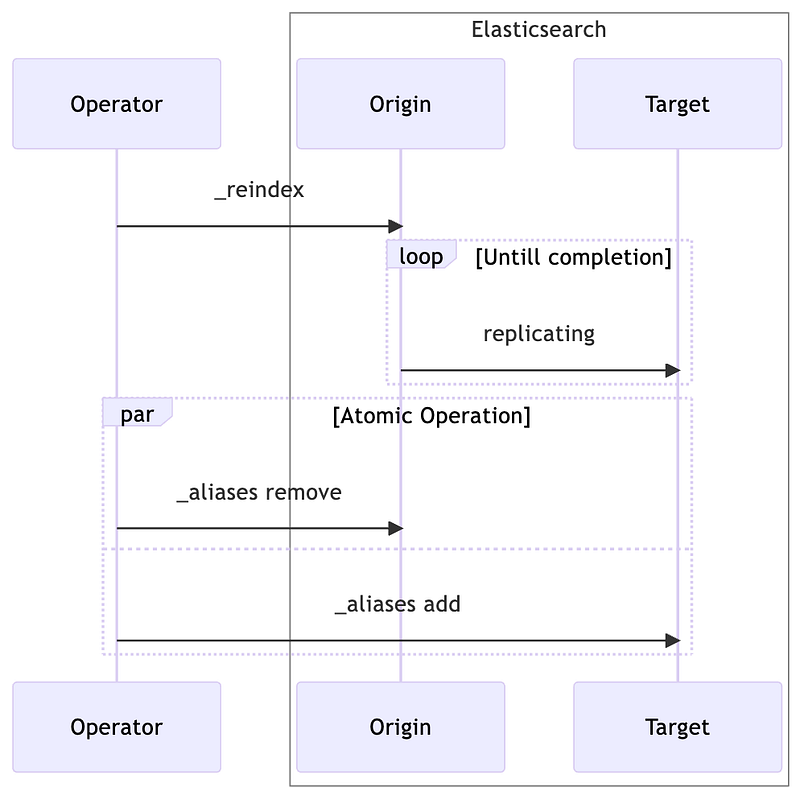
Let’s take a regular _reindex as an example. Suppose we have created an alias on the index. If we don’t have an alias, we’re in big trouble.

A regular _reindex procedure is divided into two steps.

1. Call the _reindex command to start data migration.
2. When the data migration is complete, call the _aliases command to switch between the old and new indexes.

After step 2, the new index is officially operational, and will be responsible for all read and write requests. However, this is a perfect ideal scenario, in reality, things won’t work out that way.

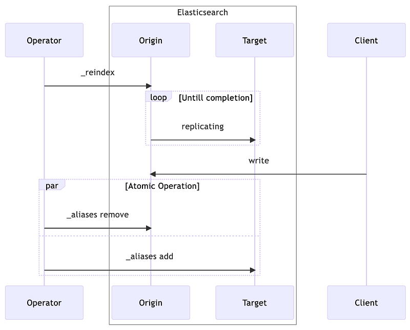
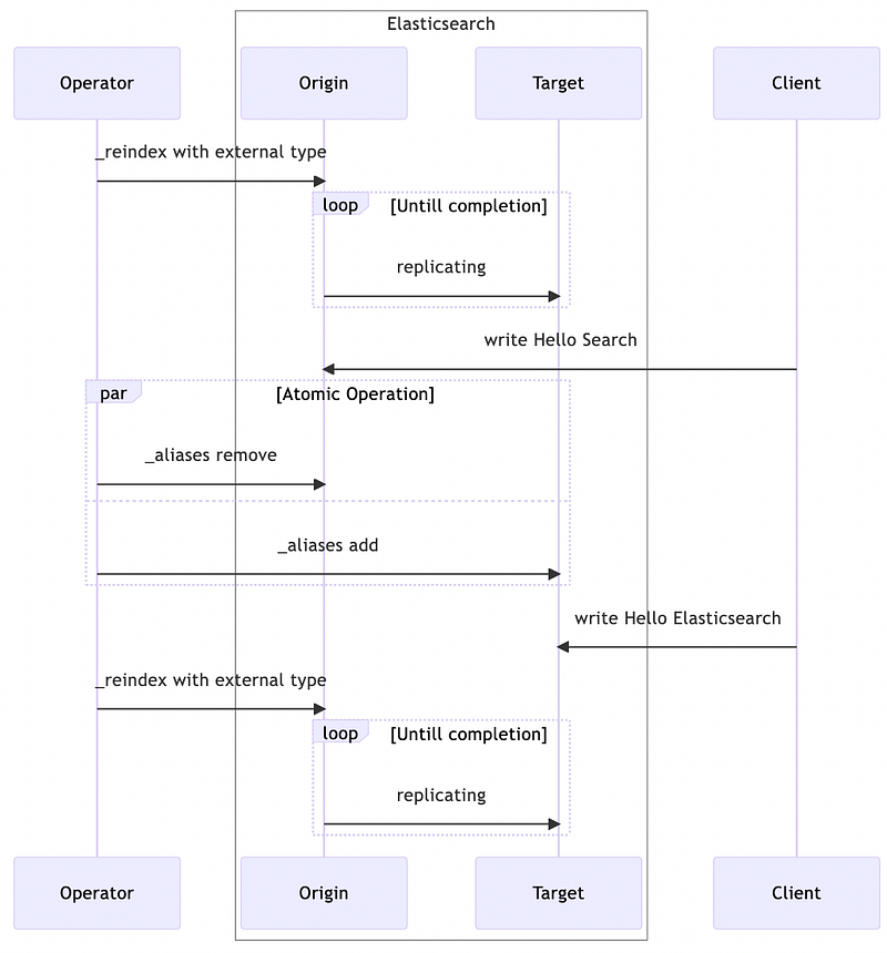
Here is a normal scenario.

Actually, during the data migration period or before switching aliases, the client will continue to write data to the original index, and these new changes will not be migrated to the new index, which leads to data inconsistency.

For the client, the feeling is that after changing the alias, all the changes just made will disappear. Furthermore, as I just mentioned, a big index migration can take hours, so the client’s feeling must be obvious.

So what to do?

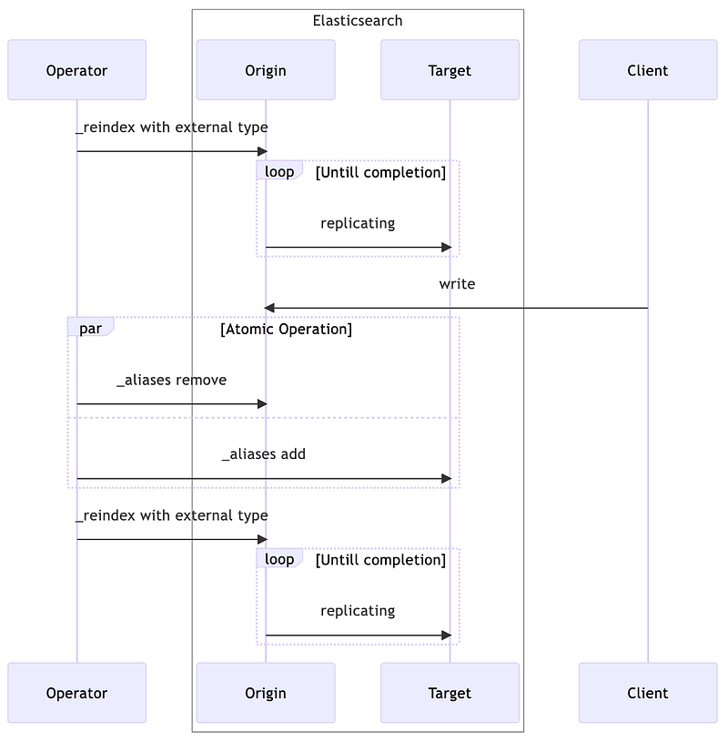
The correct flow of Reindex

The above flow makes two changes to the original flow.

1. _reindex must use external type.
2. _reindex is needed again after switching aliases.

Let’s explain the concept of the external type.

By default, _reindex is internal, and such data migration is done by using the original index to overwrite the new index anyway, and dropping the _version of the documents, so all documents in the new index start over.

If using the external type, the _version of the documents will be carried over to the new index during data migration, then the _version will be compared if there is a conflict between the _id of the old and new indexes. Only if the version of the original document is greater than the destination document will be overwritten.

A bit abstract? Let’s take an example.

Let’s say the original index has a document like the following, with Elasticsearch metadata at the beginning of the underscore.

1
2
3
4
5

{  
    "_id": "1",  
    "_version": 1,  
    "data": "Hello Elastic"  
}

When we do external data migration, _version: 1 is also written to the new index. if someone changes the original document to Hello Search during the data migration period, then the complete document will look like the following.

1
2
3
4
5

{  
    "_id": "1",  
    "_version": 2,  
    "data": "Hello Search"  
}

A redo of _reindex will find 2 > 1, so it will be overwritten with Hello Search.

Then, what if the second _reindex has someone modifying the documents in the new index? For example, if someone changes Hello Elatic to Hello Elasticsearch in the new index, will it be overwritten with the old value? The whole process would look like below.

The answer is no, because the original version has to be greater than the new version to be overwritten, if they are equal (both 2) then they are not affected.

One more problem.

Although we will do a second _reindex to patch the data, if the patch time is very long, it will still be inconsistent for the users. There are two ways to shorten the reindexing time.

1. Minimize the time of the first _reindex as much as possible.
2. Filter the patch data in advance.

Regarding the first point, the _reindex process is controlled by Elasticsearch, what else can we do to improve efficiency? Hey, there is.

We can modify the settings of the new index to minimize the IO overhead during data migration.

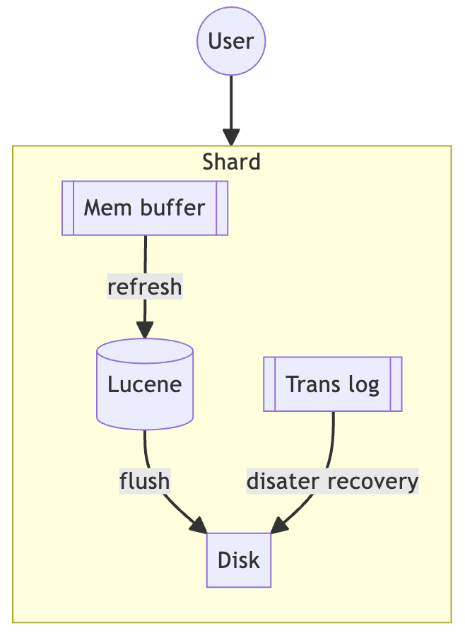
1. refresh_interval = -1
2. number_of_replicas = 0

It’s quite straightforward. First of all, the purpose of turning off refresh_interval is to allow the data migration period to just focus on writing to the Trans log and not spend extra disk IO on Lucene.

Secondly, turning off number_of_replicas reduces the additional data replication overhead that the cluster has to deal with.

On the other hand, in addition to reducing the time of the first _reindex, some data filtering can be used to reduce the amount of data for the second _reindex.

For example, bringing in the last update time of the data during the _reindex is a possible solution. Assuming that each document has an updated_at field, then adding the following condition to the query of the _reindex would be effective.

1
2
3
4
5

{  
    "range": {  
        "updated_at": { "gte": "now-1d"}  
    }  
}

Conclusion

Based on the above mentioned details, let’s list out the ideal flow of a reindex.

1. Create the destination index.
2. Update the settings of the destination index. (refresh_interval = -1 and number_of_replicas = 0)
3. Use external type for _reindex.
4. Switch aliases from original index to destination index.
5. Do _reindex again using external type, preferably with additional filtering.
6. Update the destination index setting again. (refresh_interval = null and number_of_replicas = null)

According to the official document, setting to null allows to restore the original setting.

Because _reindex is unavoidable, it is important to know how to do _reindex without downtime.

In fact, with Elasticsearch’s streaming index, there are more elegant ways to get it done. However, there are a lot of limitations on the use case for a streaming index, so it’s more common to use a regular index in practice.

This article provides a complete procedure to do _reindex as fast as possible and minimize the time of data inconsistency. However, all of this assumes that the alias is properly created, and if it is not, then more extra steps are required. I feel the lack of aliases is already a violation of Elasticsearch’s best practices, so this article doesn’t specifically cover that scenario.

Stackademic

Thank you for reading until the end. Before you go:

• Please consider clapping and following the writer! 👏
• Follow us on Twitter(X), LinkedIn, and YouTube.
• Visit Stackademic.com to find out more about how we are democratizing free programming education around the world.

Originally published on Medium

Getting Started with Flink SQL, Apache Iceberg and DynamoDB Catalog

Navigating Flink SQL, Apache Iceberg, and DynamoDB Catalog for a Lakehouse Experience

Due to the technology transformation we want to do recently, we started to investigate Apache Iceberg. In addition, the data processing engine we use in house is Apache Flink, so it’s only fair to look for an experiment environment that integrates Flink and Iceberg.

The purpose of this experiment is simply to experience using Flink SQL to operate Iceberg, but I didn’t realize that it would be so difficult to set up the whole environment.

Actually, Iceberg’s official document has a “large” description of the integration with Flink, but it is based on Hadoop and Hive. For a data engineer who has not experienced the legacy Hadoop ecosystem, Hadoop is like an abyss, and obviously the official documents don’t work.

So I referred to Dremio’s article, fixed a few fatal flaws in the article, and finally built an experiment environment where I could experience the full Flink Iceberg integration. Moreover, it’s completely local and free of charge.

Before introducing the environment, let’s quickly introduce Iceberg.

A short introduction to Iceberg

Apache Iceberg is one of the three types of lakehouse, the other two are Apache Hudi and Delta Lake.

Lakehouse, in a nutshell, is to provide a layer of interface for Object Storage that can be operated by SQL, so that lakehouse has more structured data than data lake and has the ease of use of a data warehouse.

In addition, lakehouse also provides integration with major common data processing engines, so we can enjoy the low cost of Object Storage but at the same time make the data easy to use.

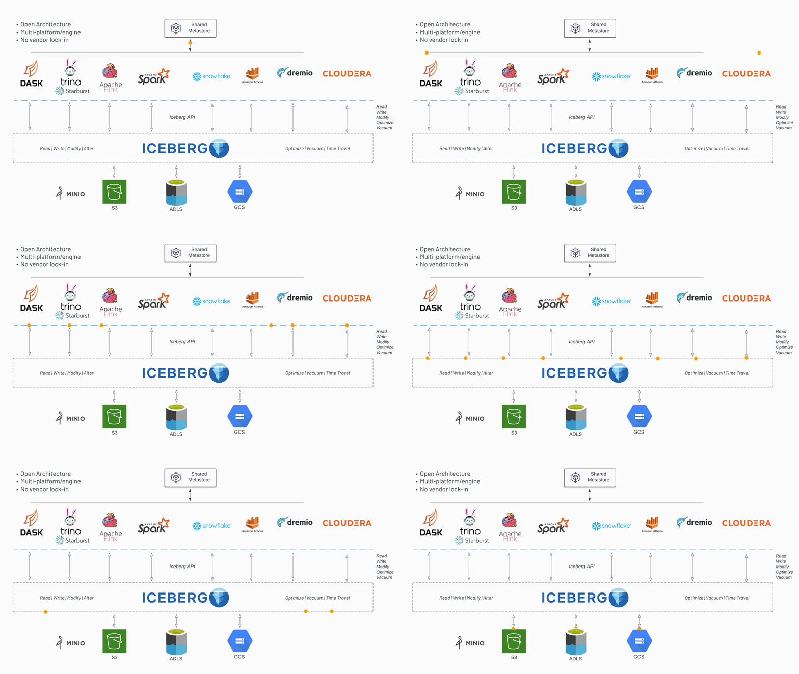
Here’s a diagram that I found very impressive.

Comparison of the three types of lakehouses is not the point of this article, there is a detailed benchmark in Kyle Weller’s article.

Experiment environment

After reading the above introduction, we understand in order to be able to perform structured data operations on Object Storage, we need a mechanism to store a schema, which is called a catalog on Iceberg.

Iceberg provides a number of options for implementing catalogs, including the Hive metastore mentioned at the beginning, and DynamoDB, which will be used in this article.

The entire playground is completely free, and at its core are the following three components.

1. DynamoDB: This is the catalog store, and uses the local version to avoid expenses.
2. Minio: This is where the actual iceberg is stored, again using minio to avoid the expense of s3.
3. Flink: the key to Playground.

The entire experiment environment has been in Github, you can clone to follow the steps.

The journey of experimentation

This environment is extremely easy to use, all you have to do is docker-compose up -d and you’re good to go.

But to get it working, I looked at a lot of articles and found that none of them actually worked, either they were buggy or just provided snippets, so I set out to make one myself.

I especially want to talk about Dremio’s article, it inspired me a lot. The only difference is that it uses Nessie as the catalog, and I’m not familiar with Nessie at all, so I used DynamoDB instead.

On the other hand, about DynamoDbCatalog, there is poor information on the Internet, not even what parameters need to be modified, I finally found out by reviewing the following source code.

Changing DynamoDB’s table name should be important if the environment goes to production, but even this parameter (dynamodb.table-name) has to be found in the code.

In addition, because the experiment environment enabled minio as an alternative to s3, there is another parameter besides endpoint that is also critical, and it requires a change in the path style approach, and again, this parameter (s3.path-style-access) is what I found by looking at the source code, which is completely undocumented.

Finally, the experiment environment has been built, there is a docker image that has been packaged with Flink and all the dependencies that need to be built, the image is a bit large and needs to be built for a period of time, so I also provide a ready-made one.

Just replace the image used by sql-client in docker-compose.yml.

Originally published on Medium

Agile Evolution: Beyond Methods

Why the Agile Manifesto author said Agile is dead

Recently, I reviewed “Agile is dead” by Dave Thomas, one of the authors of the Agile Manifesto, and after a few years of reviewing it again, I still have some new insights because of my different role (from developer to architect).

While the topic is “Agile is dead,” a more accurate statement is that Agile has survived in a wrong form. Agile hasn’t died; it’s merely subsisting.

Back to the root of the problem, Agile is essentially a spirit, a concept, or more precisely, an adjective rather than a noun. Thus, the essence of an Agile development process lies in the development process itself, not in Agile methodologies. The key is not in frameworks like Scrum, Kanban, or various other methodologies but in how to get things done quickly.

With this understanding, we realize that achieving speed in work varies based on organizational structure and existing practices. Therefore, any “general rules” provided by Agile experts or books lack reference value because:

• No rules are universal.
• All rules need context.

There are no one-size-fits-all rules; Agile practices should be adjusted according to the needs of the organization. Agile is not something that can be achieved by hiring a consultant for a short period of time, the key is to find a reasonable direction of evolution by grasping the spirit of Agile.

The conclusion of the entire talk can be summarized as follows:

• Agile is not about what you do.
• Agility is about how you do it.

Translated into concrete steps (not specific processes), it might be the following process:

1. Identify the problem.
2. Review historical experiences.
3. Make small adjustments and observe the results.

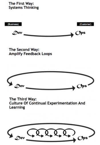
In fact, this aligns the familiar DevOps’ The Three Ways.

Additionally, the talk introduces another compelling point, especially given my current role as an architect:

• Don’t let the turkeys get you down.
• All experts are turkeys.

When I was a developer before, I used to dislike authoritative figures coming in to give directions and then leaving after stirring up the situation. They were always clean-cut, directing those in the mud from the safety of the shore. Thus, now as an architect, I try to avoid making the same mistake.

Most of the time, I provide a few suggestions and highlight the pros and cons of various solutions based on the context, allowing the engineering team I collaborate with to have a blueprint. But they need to weigh it against their own measurements themselves. Because, in the end, I am also a turkey.

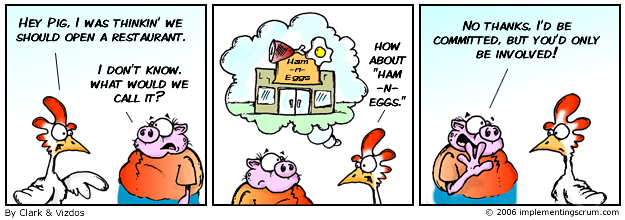
This also echoes the commonly mentioned chicken and pig story in Agile.

Originally published on Medium

這篇是翻譯Netflix最近釋出的Psyberg系列文，同時也會補充一些相關的資訊。

最主要的出處是以下三篇：

• Streamlining Membership Data Engineering at Netflix with Psyberg
• Diving Deeper into Psyberg: Stateless vs Stateful Data Processing
• Psyberg: Automated end to end catch up

Navigating Breaking Changes with Unified Queries and Gradual Schema Upgrades

When we are using a relational database, we often use incremental ID as the primary key (e.g. AUTO_INCREMENT in MySQL or SERIAL in Postgres), have you ever thought about what will happen if the incremental ID is used up?

For example, Postgres raises the following error.
ERROR: nextval: reached maximum value of sequence "<table_name>_<pk>_seq".

Don’t feel hard of happening, it is possible to accidentally set the primary key to SERIAL instead of BIGSERIAL, and then a value larger than 2147483647 will overflow. For a database, it’s not a big number.

If such a problem unfortunately occurs, what should we do to solve this?

There are a lot of articles on how to migrate data from the original table to a new table, but in fact, I don’t recommend it. Of course, it’s easiest to migrate all the data to a new table at once, but there are several problems like the following.

1. Migrating a large volume data consumes a lot of database resources, and will have a significant impact on the production environment.
2. Data inconsistency is inevitable during the migration process. For example, if data is migrated to a new table and then a new version of application is deployed to read and write the new table, if there is data written to the old table during the migration period, then there will be inconsistency.
3. If there is a downstream application that listens for updates to the source database (or CDC), then the downstream application will be flooded with events.

Therefore, I recommend that applications support both old and new tables. Creating new data is always written to the new table, but reading or updating is done according to whether the data is in the old table or the new table.

But how? For querying, should I look for the new table first and then the old table as in the example below?

1
2
3
4
5
6

if (ret := find_orig_table(params)) is not None:  
    return ret  
elif (ret := find_new_table(params)) is not None:  
    return ret  
else:  
    return None

Actually, there is an even simpler approach.

Solution Detail

To better describe the solution, let’s prepare the test environment with Postgres.

1
2
3
4
5
6
7
8
9
10
11
12
13

CREATE TABLE table_with_auto_increment (  
    id SERIAL PRIMARY KEY,  
    common_column1 VARCHAR(50),  
    common_column2 INTEGER,  
    common_column3 TEXT  
);  
CREATE EXTENSION IF NOT EXISTS "uuid-ossp";  
CREATE TABLE table_with_uuid_primary_key (  
    id UUID DEFAULT uuid_generate_v4() PRIMARY KEY,  
    common_column1 VARCHAR(50),  
    common_column2 INTEGER,  
    common_column3 TEXT  
);

Above is an old table (table_with_auto_increment) with SERIAL as primary key, it is easy to overflow, so we want to replace it with a new table (table_with_uuid_primary_key) with UUID as primary key.

There is a lot of debate on whether UUID as primary key is good or bad, but that’s not the point of this article, it’s just one of the examples.

Based on such a table structure, it will have a DTO (data transfer object) similar to the following.

1
2
3
4
5
6
7

from dataclasses import dataclass  
@dataclass  
class DTO:  
    id: ...  
    common_column1: ...  
    common_column2: ...  
    common_column3: ...

The DTO will be the same whether using the new table or the old table, so the business logic does not have to be modified during the migration process.

Then, what’s the problem of looking for the new table first and then the old one? The main problem is twice accessing the database is two round trips, which leads to one more expense, and secondly, the two functions also have maintenance complexity. Therefore, it would be great if there is a way to use one database access to assemble a DTO from two tables.

The first idea was to use UNION. However, it is worth mentioning that UNION requires both tables to have exactly the same datatype, and the id of our old and new tables are of different types.

Therefore, we need to convert the id type at the same time with UNION, and converting both of them to text is the simplest way. This is done in the following example.

1
2
3
4
5
6
7

SELECT id::text, common_column1, common_column2, common_column3  
FROM table_with_auto_increment  
WHERE common_column1 = 'test' AND common_column2 = 123  
UNION ALL  
SELECT id::text, common_column1, common_column2, common_column3  
FROM table_with_uuid_primary_key  
WHERE common_column1 = 'test' AND common_column2 = 123;

Our search criteria is common_column1 is test and common_column2 is 123, so we search both tables directly and combine the results. In general, only one of the two tables will have data ( with no bugs ), so it is very efficient to create the DTO in this way.

In this example, the purpose of creating two tables is to change ids seamlessly, so we can simplify the process through type conversion.

However, there are other scenarios where our functionality iteration leads to breaking change, so we make two tables to allow the old application to gradually transition to the new application, it may not be possible to simply do type conversion (maybe the types are not compatible at all).

So, we can consider to use OUTER JOIN method, and use the common field as the key of JOIN, so that the result will be the union of the fields of the two tables.

1
2
3
4
5
6
7
8
9
10
11
12
13
14

SELECT  
    t1.id AS t1_id, t2.id AS t2_id,  
    COALESCE(t1.common_column1, t2.common_column1) AS common_column1,  
    COALESCE(t1.common_column2, t2.common_column2) AS common_column2,  
    COALESCE(t1.common_column3, t2.common_column3) AS common_column3  
FROM  
    table_with_auto_increment t1  
FULL OUTER JOIN  
    table_with_uuid_primary_key t2  
ON t1.common_column1 = t2.common_column1 AND t1.common_column2 = t2.common_column2  
WHERE  
    t1.common_column1 = 'test' AND t1.common_column2 = 123  
OR  
    t2.common_column1 = 'test' AND t2.common_column2 = 123;

The above example is very similar to UNION, we need to find out common_column1 is test and common_column2 is 123 in two tables, but we need to list the remaining columns.

Nevertheless, the whole SQL is a bit annoying, such as the series of COALESCE, so I suggest some template rendering to make the development more intuitive.

Here’s an example of using Python with jinja2.

1
2
3
4
5
6
7
8
9
10
11
12
13
14
15
16
17
18
19
20
21
22
23
24
25
26
27
28

from jinja2 import Template  
columns = ['common_column1', 'common_column2', 'common_column3']  
template_str = """SELECT  
    t1.id AS t1_id, t2.id AS t2_id  
{% for column in columns %}  
    , COALESCE(t1.{{ column }}, t2.{{ column }}) AS {{ column }}  
{% endfor %}  
FROM  
    table_with_auto_increment t1  
FULL OUTER JOIN  
    table_with_uuid_primary_key t2  
ON t1.{{condition_column1}} = t2.{{condition_column1}} and t1.{{condition_column2}} = t2.{{condition_column2}}  
WHERE  
    t1.{{condition_column1}} = '{{condition_value1}}' AND t1.{{condition_column2}} = {{condition_value2}}  
OR  
    t2.{{condition_column1}} = '{{condition_value1}}' AND t2.{{condition_column2}} = {{condition_value2}};  
"""  
condition_column1 = 'common_column1'  
condition_column2 = 'common_column2'  
condition_value1 = 'test'  
condition_value2 = 123  
template = Template(template_str)  
query = template.render(  
    columns=columns,  
    condition_column1=condition_column1, condition_column2=condition_column2,  
    condition_value1=condition_value1, condition_value2=condition_value2  
)  
print(query)

At this point, we’ve been able to make the transition from the old table structure to the new one seamless for the application.

Conclusion

Although in this article we have introduced how to solve the problem of id exhaustion, it can be used in any scenario where we need to make a breaking change to the table structure of the database.

When the data volume is small, breaking change is not a big deal, we just need to migrate all the old tables to the new ones, but when the data volume is huge, such an approach will increase a lot of operation risks.

A complete table migration involves not only the data migration itself, but also how to keep the production environment unaffected. The most common problem we encountered is how to synchronize the data to the new table if there are still clients writing to the old table during the data migration period.

In addition, in order to avoid affecting the production environment, we usually have to choose the off-peak time to perform the migration, which inevitably requires many departments to work overtime together.

For instance, the development team needs to release a new version of the program, the operation team needs to migrate the data, the SRE team needs to monitor the risk of online, and the QA team needs to validate. It is not worth for me to work so hard just for the sake of table migration.

Therefore, it’s best to be able to upgrade your application to a new version seamlessly. This article introduces a simple but effective practice to avoid many unnecessary breaking changes. Of course, there are many different ways to achieve this, if you have some good solutions, please feel free to share them with me.

Stackademic

Thank you for reading until the end. Before you go:

• Please consider clapping and following the writer! 👏
• Follow us on Twitter(X), LinkedIn, and YouTube.
• Visit Stackademic.com to find out more about how we are democratizing free programming education around the world.

Originally published on Medium

Handling Stale Sets and Thundering Herds of Cache

Simplified Approach Inspired by Facebook’s Innovative Solution

Recently, I’ve been studying how Facebook handles caching at scale, and one of the subsections describes how they handle stale sets and thundering herds. They use a lease mechanism to face these two problems at once, which is very interesting.

What are stale sets and thundering herds? Let me explain each in one simple sentence.

• Stale sets: Data inconsistency between cache and database.
• Thundering herds (aka Dogpile effect): High concurrency request to knock down the database.

In fact, I have also introduced how to solve the problem of stale sets and thundering herds, only that I have proposed my own solutions to each problem, and I do not have a one-size-fits-all solution.

• Solving stale sets
• Solving thundering herds

Let’s take a look at how Facebook solved two problems at once.

Problem Description

First, let me briefly explain the two problems.

In general, the behavior of a read-aside cache is to read from the cache first, and if it can’t be found, then read from the database instead. After retrieving data, write the data back to the cache. If the database is updated, the cached data is cleared without writing it back.

Even with this process, there are still problems, the most typical of which are the two problems mentioned in this article. The process of how stale sets occur is as follows.

Although B has cleared the cache, A is delayed for “some reason”, so the data in the cache is written to the old data, which is the data stale or inconsistent.

On the other hand, when a cache miss occurs in a highly concurrent system, then all these clients will query the database, in other words, the database will fall down in a short time due to high concurrency. This problem is also known as the Dogpile effect.

Facebook’s solution

How did Facebook solve these two problems? They use a lease mechanism, which is described in section 3.2.1 of the paper, but the explanation is not very complete, it is roughly the following two paragraphs.

A memcached instance gives a lease to a
client to set data back into the cache when that client experiences a cache miss. Verification can fail if
memcached has invalidated the lease token due to receiving a delete request for that item.

And.

We configure these
servers to return a token only once every 10 seconds per
key.

When writing data to the cache, it must carry the token that was obtained during the cache miss. The cache will first validate the token before updating, and if the token validation fails, then it will be ignored. The token will be cleared when the database is updated.

Let’s explain this with the sequence diagram.

The difference between this diagram and the problem one is the first interaction will get a token, when write cache need to carry the token, but because the token has been cleared after updating the database, so write cache will be rejected, this will solve the first problem.

As for the second problem is not difficult to deal with, just need to set the rules for the token release, every 10 seconds to send a token, if the client does not get the token then there is no authority to update the cache naturally there is no need to query the database, the Dogpile effect can be solved.

Simple implementation

To implement this logic is not so difficult, let’s use Python and Redis to write a simple example.

1
2
3
4
5
6
7
8
9
10
11
12
13
14
15
16
17
18
19
20

class Cache:  
    def __init__(self):  
        # ignore implementation  
    def get(self, k):  
        v = self.redis.get(k)  
        token = random.getrandbits(64) # Facebook says the token has to be 64 bit.  
        ret = self.redis.set(f'{self.prefix}#{k}', token, 'NX', 'EX', 10) # 10s for token refresh  
        return (v, token if ret == 'OK' else None)  
  
    def set(self, k, v, token):  
        saved_token = self.redis.get(f'{self.prefix}#{k}')  
        if token == saved_token:  
            ret = self.redis.set(k, v)  
        else:  
            ret = False  
              
        return ret == 'OK' or False  
      
    def clean(self, k):  
        self.redis.del(k, f'{self.prefix}#{k}')

To make it easier to understand, here we only show the core implementation and do not use Lua or other pipeline optimization methods.

In get, two values are returned, one is the result of the cache and the other is the token, if the original token still exists and has not expired, which means there is a possibility of thundering herds, then the token is not returned, and if the client does not receive the token, then he should not query the database.

In set, in addition to the key and value to write, we also need to carry the token, when the validation of the token fails, we don’t update the cache and just end it so as to avoid stale sets.

Conclusion

Stale sets and thundering herds are pretty common problems when using caches, and there are many solutions for them. But when I actually wrote the program based on Facebook’s solution, I realized that it can be so simple, which made me a bit surprised that we were “overthinking” before.

I believe that the simpler the solution, the better, and I will use Facebook’s solution to deal with the problem at hand in the future. In fact, there are many more methods and optimizations for dealing with caching at scale in this paper, making it a very worthwhile study.

Originally published on Medium

Exploring Three Viable Approaches to Optimize Database Resources

There are always times when the available space in the database is exhausted, and we need to take action.

Generally, the most common approach is vertical scaling, also known as scale-up, which involves increasing the specifications of the machine directly to expand the available space. Another alternative solution is horizontal scaling, also known as scale-out or sharding, which enhances overall available space by distributing data across different machines.

However, both scale-up and scale-out involve costs, and these can be substantial. For organizations with budget constraints, neither of these approaches may be immediately feasible. So, what can be done?

In such cases, the only option is to squeeze out as much space as possible from the existing machines, no matter what it takes, just pure squeezing.

In this article, we take MongoDB as an example to explore the viable approaches for squeezing out available space.

Remove useless index

Indexes are a trade-off of space for time to improve query performance. Therefore, if unused indexes can be identified and removed, the initially consumed space can be reclaimed.

Why do indexes become redundant?

There are several common reasons as follows:

1. Because MongoDB’s WiredTiger is a B-tree-based storage engine, it has a feature known as the leftmost-prefix. Thus, if a new index and an old index have the same prefix, the old index can be safely removed without affecting query performance.
2. Due to feature iterations, some queries that were required initially are no longer in use.

Regarding the first point, we can easily identify which indexes can be removed by carefully scanning each index. However, for the second point, some additional preparation is necessary.

We need to know which indexes are not being used. Apart from tracing clues from the code, there is a more efficient approach, which is to directly examine the index metrics. In the case of MongoDB, the $indexStats aggregation operation can provide statistical data on the indexes.

By comparing the statistics from two time periods, we can determine which indexes are not being used.

Remove useless data

The above-mentioned approach of deleting indexes is a relatively straightforward solution that does not affect the production environment. However, if more available space needs to be squeezed out, consider deleting unused data.

Defining what constitutes unused data entirely depends on the application. For instance, some applications use flags to mark softly deleted documents, allowing these softly deleted documents to be removed or archived to cold storage.

Another scenario involves time-series data, where defining how old the data should be before it can be deleted becomes relevant. However, whichever solution is chosen depends entirely on the application.

Reshard

This is a more advanced approach compared to the previous two, directly impacting the performance of the production environment.

If the MongoDB cluster is already a sharded cluster but some collections have not been sharded, setting the appropriate shard key and enabling sharding can be a relatively straightforward process.

However, if all collections have already been sharded, it’s essential to examine which collections have uneven data distribution. Consider modifying the shard key and even taking further steps to rebalance. Phew, as of MongoDB 5.0, we can finally reshard a collection.

I previously wrote an article describing how to correctly design a shard key to achieve as even a data distribution as possible.

We can determine whether data distribution is uniform by using the command sh.status(). This command provides explicit information in the output regarding how many shards are being used for a collection and how many chunks each shard holds. A chunk represents the unit of data distribution.

However

It seems like we have several approaches that should all be effective if carefully implemented, right?

In reality, after implementing the second and third approaches, observing the available space reveals no improvement. In fact, it may even worsen, especially after executing the third approach.

The following diagram illustrates the usage space of a particular shard on the y-axis over time on the x-axis. Here, t1 denotes the initiation of sharding, while t2 represents the completion of the sharding process.

We aimed to shard a collection that had not been sharded yet to release the available space in the original shard. However, as we can see from the diagram, after the sharding process was completed, the situation worsened, which was entirely contrary to our expectations.

Why did this happen?

The reason lies in WiredTiger’s behavior. After deleting documents, it does not immediately release the space. Instead, it retains the already allocated space, ensuring prepared chunks for future data writes in the collection.

This intention is well-meaning, as disk I/O performance is poor, and having a pre-arranged “clean slate” is valuable. However, this contradicts our goal of having the data disappear immediately after deletion. Hence, we see that although data is deleted, the available space does not increase.

Why did the diagram not only fail to decrease but also grow?

During the sharding process, to enable more efficient sharded queries, an index is created on the shard key. The additional space consumption represents the space occupied by these indexes.

Can we determine how much space WiredTiger has covertly consumed? The answer is yes.

Executing the command db.collection.stats() yields an output segment that describes “file bytes available for reuse,” representing the space that has been covertly taken.

If we can find it, we can certainly reclaim it. Running the compact command accomplishes this. It’s worth noting that the space regained through compact can only be used by the same collection, so the problem remains unresolved.

To enable all collections to reuse the occupied space, a complex procedure is required. Let me simplify the explanation.

When we add a new member to a ReplicaSet in MongoDB, the new member executes an Init Sync to synchronize the current data. However, this Init Sync only synchronizes actual data and not the occupied space. In other words, the new member does not occupy the available space.

Thus, if we gradually replace all the members in a ReplicaSet, we can obtain a new cluster (or Ship of Theseus) with the same dataset but without the occupied space. However, this process requires a “slight” additional budget to enable an extra machine as a new member, which is no longer necessary after the entire replacement process is complete, resulting in significant savings compared to scaling up or scaling out.

Conclusion

For any organization, finances are always a significant concern, particularly when it comes to database expenses, which can be quite substantial. While we aim to minimize costs wherever possible, the options available to us are limited. However, let’s quickly summarize the three methods to squeeze out available space:

1. Remove useless indexes
2. Remove useless data
3. Reshard

These three methods are in his order of precedence, with the first one being the quickest to implement and having the least impact on the production environment, and vice versa.

Moreover, executing solutions 2 and 3 requires additional processes to ensure that the space is genuinely available and not occupied.

Perhaps there are some secret techniques that I haven’t thought of yet. Feel free to share them with me.

Originally published on Medium