CT Wu

Generative AI transforms the way we handle business logic

• Paradigm Shift in Software Development, Part 1
• Paradigm Shift in Software Development, Part 2

If you read the title and thought I am going to introduce Copilot, you are wrong.

Before we start the topic, let’s start with a case study of an e-commerce platform.

Suppose the shopping cart looks like the following.

1
2
3
4
5
6
7
8
9
10
11
12
13
14
15
16
17
18
19
20

[  
  {  
    "product_id": 123,  
    "amount": 2,  
    "price": 10.99,  
    "category_id": 1  
  },  
  {  
    "product_id": 456,  
    "amount": 1,  
    "price": 29.99,  
    "category_id": 2  
  },  
  {  
    "product_id": 789,  
    "amount": 5,  
    "price": 1.99,  
    "category_id": 3  
  }  
]

Each field should be simple enough to contain the item purchased, the quantity purchased, the price of the single item, and the category it belongs to.

I have 3 promotions.

1. $5 off a $20 purchase, which continues to accrue after qualifying.
2. buy 2 get 1 free on category_id 1 items.
3. 30% off the total price of category_id 3 items.

• What is the total price after calculation?
• How much of the discount is allocated to each item?

To implement such promotions, please answer the following questions.

• How long would it take you to implement this logic?
• Can you make the logic better than O(n²)?

The first question is easy to understand, but what does the second question mean?

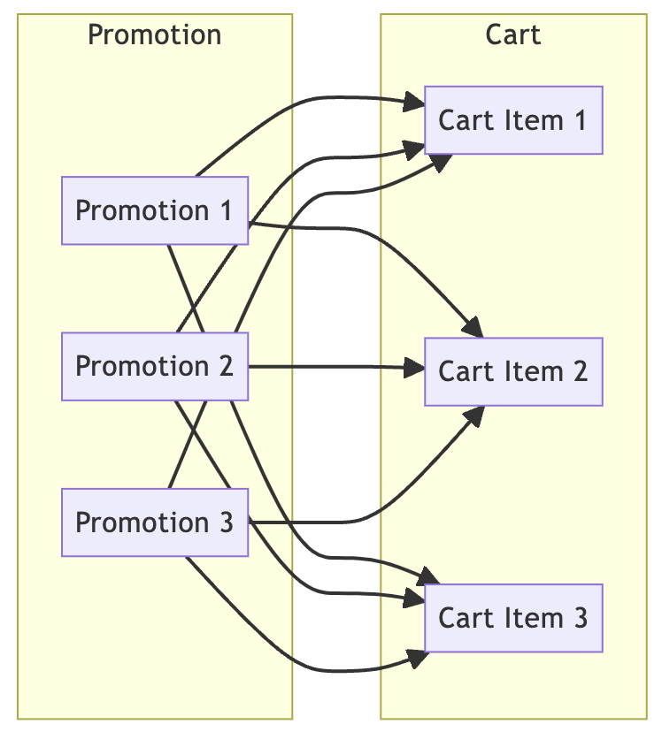
We have three promotions, and to be able to determine the impact of every promotion we need to scan the entire shopping cart for every item. So, in the example above, that’s 3 * 3 = 9, i.e. O(n²).

Then

What if I told you:

• I could do it in just a few minutes.
• And it’s O(1).

Would you believe me?

Guess how I did it.

GenAI can help

Although GenAI was mentioned, if you thought I am going to introduce Copilot or similar tools, you are very wrong.

It’s true that those code generation tools can produce business logic in a matter of minutes, but the business logic they produce will still work the way we think, which means it will still be O(n²).

So what do we do with GenAI? The answer is simple: let GenAI learn business logic and then answer the results directly.

Sounds unbelievable, right? Let’s see how I did it.

GEMINI DEMO LINK (a google account required.)

Even though I’m using Gemini as an example, actually, you can use any model.

Step 1

First, I’ll tell Gemini his role using System Instructions.

You are an e-commerce expert who is well versed in all kinds of promotions and understands how shopping cart profits are calculated.

Step 2

Next, ask Gemini to explain the structure of a shopping cart that I dropped in. It’s important to ask him to explain this. Instead of telling him what it is, it’s better to let him understand it for himself so that he can get a more accurate mental model.

Let’s describe a shopping cart in JSON, here’s an example.

Step 3

Tell Gemini what he needs to know about the promotion, and explain in detail what we need. This echoes the question at the beginning of this article. The point of this step, by the way, is not just to explain the promotion, but also to tell him what results to send back.

Step 4

Based on Gemini’s thought process, we have to keep correcting it until his understanding and calculations are correct. Fortunately, GenAI doesn’t hide anything. He tells us step by step what he’s thinking, so it’s easy to find mistakes in the middle. I have to say, it’s much easier to debug a natural language than a programming language.

Step 5

Ask Gemini to generate a response structure that corresponds to the requirements in step 3, which is why I said we should tell him what we want as early as possible. Otherwise, we may need to go back and adjust his thought process at this step, which would be ineffective.

Final step

Because GenAI will still keep “describing” his answer, we have to tell him, “I don’t want to see the process, I just want to see the result, and I don’t want any description”.

Finally, the business logic is complete.

Wait, that’s a little weird. We don’t deal with business logic this way by interacting with GenAI.

Yes, that’s right! The first step to the last step are all pre-defined “prompts”, and we can get the result by wrapping all these prompts and business logic inputs in the same question and asking GenAI.

In fact, it looks like this.

The INSERT_INPUT_HERE is actually the original structure of our shopping cart promotion calculation.

This process is exactly the same as the popular prompt engineering nowadays.

Conclusion

In this article we have shown a case study of using GenAI to accomplish business logic.

Let’s organize the whole process again.

1. Inform about the role of GenAI
2. Explain the input of the business logic.
3. Describe the requirements of the business logic.
4. Correct GenAI’s errors.
5. Generate the output of the business logic.
6. Prune all descriptive statements.

These steps are all centered around prompt engineering, and the more you are familiar with prompt engineering, the quicker the process will be.

The benefits of this process are not only that we can make O(n²) business logic processing become O(1) as mentioned at the beginning, but also that we can make business logic easier to debug. As I said, it’s much easier to catch human speech defects than it is to find bugs in a program.

Nevertheless, there is one important thing to realize about this development process. We have to realize that GenAI is actually a Large Language Model, or LLM, which is not good at computation. So when we use GenAI to write business logic, we still need to have full unit testing to make sure the results are what we expect.

In other words, the importance of unit testing increases rather than decreases with this development process.

When we think of GenAI for software development, we always think of Copilot, but it’s much simpler to let GenAI implement business logic directly without generating code.

Stackademic 🎓

Thank you for reading until the end. Before you go:

• Please consider clapping and following the writer! 👏
• Follow us X | LinkedIn | YouTube | Discord
• Visit our other platforms: In Plain English | CoFeed | Differ
• More content at Stackademic.com

Originally published on Medium

How to Determine API Slow Downs, Part 2

Understanding PELT algorithm and its applications in Change Point Detection

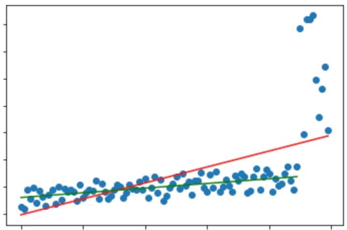
A long time ago I wrote an article on how to determine an API is slowing down using simple statistics known as linear regression.

In the conclusion of that article, it was mentioned some challenges in applying linear regression.

1. It is hard to define the reference point.
2. Difficulty in defining the angle of the regression lines.

The reference point means we need two regression lines to know whether the current situation is normal or abnormal, and the angle between the regression lines is the basis for our judgment.

For those who are familiar with statistics or math, this approach is a bit naive. In fact, I have not formally studied statistics, so I can only use the most straightforward approach, which has been proven to be feasible in practice, but the process of fine-tuning in the early stages will be tough.

After several years of continuous studies, I found a simpler way to do this, which is Changepoint Detection.

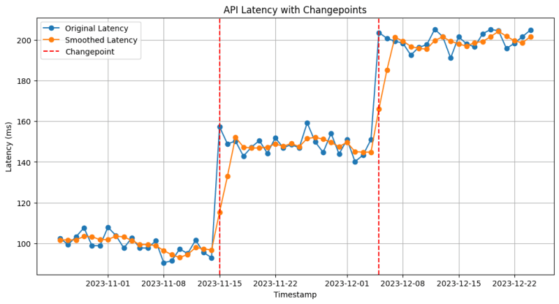
Before going into the details, let’s use a diagram to see what Changepoint Detection can do.

The source code is linked here.

As we can see from the diagram, our API slows down twice, and our tool detects the exact point in time. Although I have done smoothing here, in practice it is fine without it, only the detection thresholds need to be adjusted accordingly.

Solution Details

Originally we needed to solve two problems, but now we no longer need a reference point, so only the threshold needs to be defined. I have to say no matter what the mechanism is, thresholds are inevitable, to have an alarm is to need a threshold.

Well, let’s see how the magic happens.

1
2

model = Pelt(model="rbf").fit(np.array(df['smoothed_latency']).reshape(-1, 1))  
changepoints = model.predict(pen=5)

The source code is a bit long, but the core of the program is these two lines.

We use a famous Changepoint Detection algorithm: Pruned Exact Linear Time aka PELT. This is the algorithm proposed by Killick in 2012.

The whole process is actually three steps.

1. Decide what model to use, in this case we use rbf.
2. Feed data points into the model.
3. Predict the changes through the model.

Let’s continue to break down these steps.

How to choose the right model?

In ruptures.Pelt, there are many models (cost functions) are available, the following three are more commonly used.

l2（least squared deviation）

This model is useful mainly for scenarios where there is a change in the average and if there is a significant change in the average, then this model is good to use.

For example, if there is a significant increase in the average latency after a certain release, e.g. 100ms to 200ms, then l2 can easily capture this version.

rbf（Radial Basis Function）

rbf is more commonly used in the case of irregular variations, such as where both the average and the trend are changing.

For example, a latency in a complex system can be affected by a number of factors, and rbf can be used to find the more “subtle” changes.

normal

The term normal refers to a normal distribution or Gaussian distribution. The key to a normal distribution is the mean and standard deviation, so this is used in the context of distributional change.

For example, network traffic during peak hours not only increases in average but also in volatility, which is a kind of distributional change.

How to set the penalty?

In the second line of the code, there is a pen=5, where pen refers to the penalty.

Briefly, the larger the penalty, the tighter the model will be, and the fewer changepoints can be found, and vice versa.

So it is still a matter of experimentation as to what value to set, just as we did with linear regression, where we needed to experiment with how to define the angle of the regression lines. Even with PELT, we still need to consider how to set the penalty.

Conclusion

In fact we want to do exactly the same thing as before, we want to detect when the API is slowing down and it is slowing down because of a defect.

At first, we used the angle between the two regression lines to determine this. But this approach, as we mentioned, requires a lot of experimentation to determine how to define the reference point and the threshold of the angle. Although the concept is simple and not difficult to implement, it is not easy to make it work in practice.

In order to reduce the number of experiments, we change the factors from two to one, and only need to determine the penalty through experiments, which is a necessary process no matter what solution is used. In other words, we have greatly reduced the complexity of the API monitoring system.

You may ask, don’t we need to experiment to choose the model? No, not at all.

Because these models have a clear purpose, as long as you know what patterns you want to check, you will naturally choose the corresponding model. The reason we chose rbf is because we want to know if the API is abnormal as it slows down, which involves not only the average change but also a lot of additional factors, and only rbf is more fitting.

The source code is quite simple, the core is the two lines introduced in this article. But I have to say, to be able to write these two lines requires a huge accumulation of knowledge, and I also deeply realize that programmer is not just about writing code ONCE AGAIN.

Originally published on Medium

PostgreSQL Full-Text Search in a Nutshell

Discover how to implement efficient and powerful text search capabilities in your PostgreSQL database

If you ask me to choose a database for microservices, I would probably say PostgreSQL.

On one hand, PostgreSQL is a popular open source database with many mature practices, both on the server side and the client side. On the other hand, PostgreSQL is very “scalable”. Scalability of course includes non-functional requirements such as traffic and data volume, as well as functional requirements such as full-text search.

In the early stages of planning a microservice, we may not be sure what features it needs to have. I have to say those tutorials always telling us microservices need to have clear boundaries early in design are nonsense.

Most of the time, as a microservice goes live, there are more requirements and more iterations, and those requirements don’t care about the boundaries you define at the beginning.

Full-text search is a good example. In the early days of a service, we might be able to work just fine with a exact match or prefix match of text. Until one day, you get a request. “Hey, let’s add a search feature!”

If the database you chose in the beginning doesn’t have a search function, then that’s a big problem.

I’m sure you wouldn’t introduce a database like Elasticsearch, which specializes in full-text search, for this sudden need. So what to do?

Fortunately, PostgreSQL has a solution.

PostgreSQL Built-In Features

In the official document there is a large chapter on how to do full-text searching with PostgreSQL.

Let’s skip all the technical details and go straight to the how-to.

1
2
3
4
5

SELECT id, title, body, author, created_at, updated_at, published,  
       ts_rank(tsv, to_tsquery('english', 'excited | trends')) AS rank  
FROM blog_posts  
WHERE tsv @@ to_tsquery('english', 'excited | trends')  
ORDER BY rank DESC;

blog_posts is a table of stored blog posts, where tsv is a special column. It is not a metadata that a blog needs, it is a column that we create for searching purposes.

1
2

ALTER TABLE blog_posts ADD COLUMN tsv tsvector;  
UPDATE blog_posts SET tsv = to_tsvector('english', title || ' ' || body);

As we can see, tsv is the result set when we join title and body and do the English stemming.

The methods to_tsvector and to_tsquery are the core of this query. It is through these two methods that you can efficiently create the synonyms from the built-in dictionary. If you’re familiar with Elasticsearch, then what these two methods are doing corresponds to analyzer.

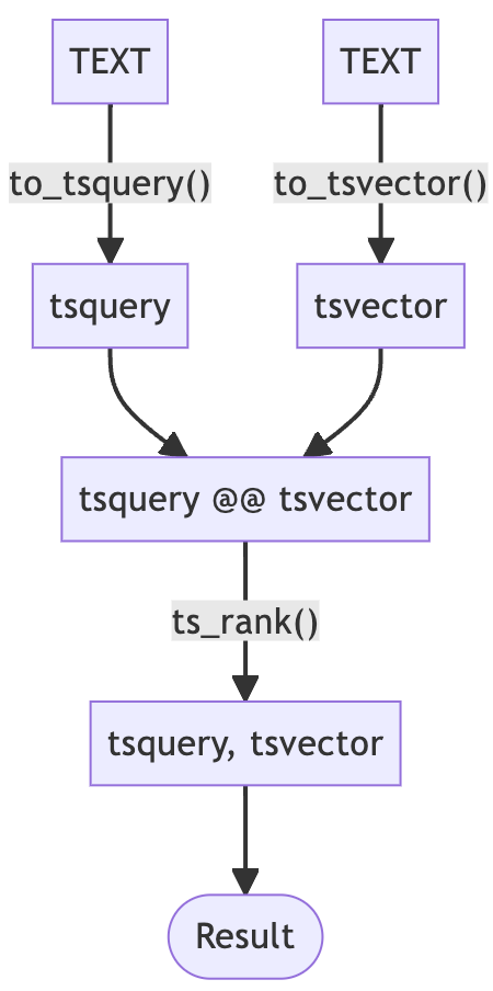
Let’s explain this with a flowchart.

The tsvector is the result that we store in advance through tokenizer and token filter operations. The same is applied to tsquery, but it is lighter. Then we compare tsquery and tsvector by using the matching operator @@, which produces a dataset containing the query results. Finally, the score is calculated and sorted by ts_rank.

In fact, the whole process is the same as what Elasticsearch does, except that PostgreSQL takes away the ability to customize and relies on the built-in dictionary.

It’s worth mentioning that the tsv column needs to be indexed with a GIN type index, otherwise the performance will be poor.

1

CREATE INDEX idx_fts ON blog_posts USING gin(tsv);

Elasticsearch is efficient not because it has a powerful analyzer, but because it uses inverted indexes at the backend. In PostgreSQL’s case, it’s GIN, Generalized Inverted Index.

Again, the technical detail is not the focus of this article, so I’ll skip it.

Non-built-in PostgreSQL catalogs

It is not difficult to list all currently supported languages for PostgreSQL.

1

SELECT cfgname FROM pg_ts_config;

As of today (PostgreSQL 16), there are only 29 in total.

1
2
3
4
5
6
7
8
9
10
11
12
13
14
15
16
17
18
19
20
21
22
23
24
25
26
27
28
29
30
31
32
33

postgres=# SELECT cfgname FROM pg_ts_config;  
  cfgname  
------------  
 simple  
 arabic  
 armenian  
 basque  
 catalan  
 danish  
 dutch  
 english  
 finnish  
 french  
 german  
 greek  
 hindi  
 hungarian  
 indonesian  
 irish  
 italian  
 lithuanian  
 nepali  
 norwegian  
 portuguese  
 romanian  
 russian  
 serbian  
 spanish  
 swedish  
 tamil  
 turkish  
 yiddish  
(29 rows)

As seen, there is no CJK language at all, i.e. there is no ability to handle double-byte characters.

For languages without built-in support, they can be handled by extensions. Take Chinese as an example, pg_jieba is a widely used extension.

After installing the extension, we just need to modify the catalog in PostgreSQL.

1
2

CREATE EXTENSION pg_jieba;  
UPDATE blog_posts SET tsv = to_tsvector('jieba', title || ' ' || body);

The above is an example of to_tsvector, and of course, to_tsquery is the same.

So languages without built-in support can find language extensions to enhance PostgreSQL’s capabilities. This is one of the great things about PostgreSQL, it has a rich ecosystem of additional features.

What about AWS RDS?

In the previous section we mentioned that we can install additional extensions to support more languages, however, AWS RDS cannot customize extensions.

In this case, we have to transfer the server-side effort to the client-side.

In other words, we need to implement the language-specific stems on the client side and write tsv on the client side.

Let’s continue with jieba as an example. This is the main program logic for pg_jieba, which is also a Python package, so let’s use Python for the example.

1
2
3
4
5
6
7
8
9

import jieba  
  
def tokenize(text):  
    return ' '.join(jieba.cut(text))  
  
cur.execute("""  
    INSERT INTO blog_posts (title, body, author, tsv)  
    VALUES (%s, %s, %s, to_tsvector('english', %s))  
""", (title, body, author, tokenize(title + ' ' + body)))

Similarly, the query is also done by jieba.cut and then to_tsquery. One interesting thing is we still use english as the catalog in this example, but it doesn’t really matter what we use. I just need the ability to split text with whitespace.

Conclusion

In this article, we can see the power of PostgreSQL.

It has many useful features and a rich ecosystem. Even if these readymade implementations are not enough, we can still implement on our own through its stable and flexible design.

That’s why I prefer PostgreSQL.

If we don’t think about something clearly in the beginning, there are many chances that we can fix it without getting stuck in a mess.

This article provided an example of full-text searching, and I’ll provide an additional interesting example. At one time, I was using PostgreSQL for a microservice and focused on its ACID capabilities. However, the requirements changed so drastically that ACID was no longer a priority, but rather the ability to flexibly support a variety of data types.

Suddenly, PostgreSQL can be transformed into a document database, storing all kinds of nested JSON through JSONB.

Thanks to the flexibility of PostgreSQL, it has saved my life many times, and I would like to provide a reference for you.

Originally published on Medium

A quick-start environment for effortless exploration and learning

Earlier I briefly introduced Apache Iceberg and built an out-of-the-box experiment environment.

The purpose of the article was to experience the integration of Flink SQL and Iceberg, so that I could quickly move on to the next stage of Flink development. Surprisingly, the article was really popular, and I received a few stars on my Github. It made me realize many people like me find these big data technical stacks tough and want a tutorial.

So, let’s welcome another big data star, Trino.

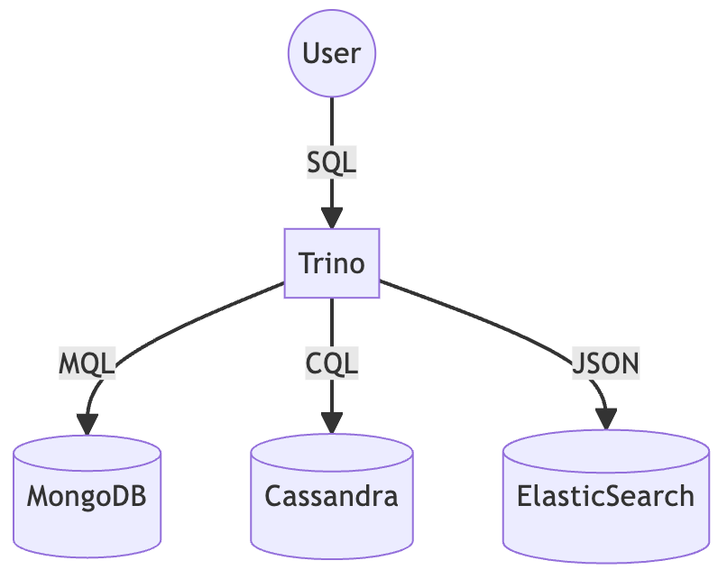
Trino is a popular query engine that provides a single entry point of access to multiple heterogeneous data sources and the ability to query them using SQL. This is a bit abstract, let’s take an example.

Even though every data source has different query syntax, Trino integrates well and interacts with users using SQL.

In addition to common databases, Trino also supports Iceberg queries. Thus, let’s experience the integration of Trino and Iceberg, and I will provide a experiment environment as well.

Experiment environment introduction

First, provide the link to the experiment environment.

Before we get started, let’s take a quick look at the basic structure of Trino, which has three layers: catalog, schema, and finally table. Let’s use MongoDB as an example, where catalog corresponds to a database cluster, schema refers to the name of the database under the cluster. As for table, it simply refers to collection.

However, the meaning of this catalog is different from that of Iceberg’s. Iceberg’s catalog is just one of Iceberg’s settings, not the one that Trino recognizes as a catalog.

Sounds confusing? Let’s look at an existing example, example.properties.

1
2
3
4
5
6
7
8
9
10

connector.name=iceberg  
iceberg.catalog.type=nessie  
iceberg.nessie-catalog.uri=http://catalog:19120/api/v1  
iceberg.nessie-catalog.default-warehouse-dir=s3://warehouse  
fs.native-s3.enabled=true  
s3.endpoint=http://storage:9000  
s3.region=us-east-1  
s3.path-style-access=true  
s3.aws-access-key=admin  
s3.aws-secret-key=password

This is a Trino catalog setup. We can see this catalog is linked to an Iceberg source. Below we specify the Iceberg-specific catalog as nessie and provide the nessie settings.

By the way, I wanted to continue to use the previous experiment with Flink SQL and Iceberg, but I found out Trino doesn’t support Iceberg’s DynamoDB catalog. Therefore, I had to create a new one.

So far we have created a catalog called example, and we will continue to build the schema and tables under it.

To initialize the tree structure, we override command in docker-compose.yaml so that the Trino container calls post-init.sh on startup.

1
2
3
4
5
6
7
8

#!/bin/bash  
nohup /usr/lib/trino/bin/run-trino &  
  
sleep 10  
  
trino < /tmp/post-init.sql  
  
tail -f /dev/null

In the script, we first wake up Trino’s original startup script, then wait for 10 seconds for Trino to initialize, and then feed the SQL we want to execute. Finally, it waits until it receives a kill signal.

Conclusion

In the data engineering world, where new technical stacks are constantly being created, it can be difficult just to play with each one once, not to mention comparing the tools.

So I hope these experiment environments will provide people who want to play around with them a quick experience without actually getting their hands dirty.

As for comparing tools, it would be great if someone had a more complete benchmark report to share with me. For example, I’d love to know, at this point in time (May 2024), what would be the best choice between the three lakehouses? Or how about Trino and Presto?

I have an answer in mind, but I’d like more objective numbers, so feel free to discuss.

Originally published on Medium

Exploring the roots and pathways to overcoming data fragmentation

Nowadays, data engineering is facing many challenges, and one of the toughest issues is the complex technical stack and the emerging problem of data silos.

The term “data silos” refers to data that is scattered in several places, which are difficult to connect and integrate with each other, as if they are isolated (and they are indeed physically isolated).

There are many reasons for data silos, for example:

• Separate data pipelines between different departments
• Data centers in different regions for compliance purposes.
• For cost reasons, technical stacks are built on different vendors.
• And so on.

The most complicated scenario in these cases would be data silos across several public clouds.

For instance, the original technical stack was built on GCP, so cloud services such as GCS and BigQuery were widely used. But then, for various reasons, we started to build AWS data stacks, so we need to use S3 and Redshift, etc. In fact, all three public clouds have similar roles in data engineering.

In fact, in the three major public clouds, there are similar roles in data engineering responsible for the corresponding functions.

If we are looking for relational databases, AWS has RDS, Azure has SQL Database, and Cloud SQL is also available on GCP. If we are looking for object storage services, AWS has the famous S3, Azure also has Blob storage, and GCP also has GCS.

If we are looking for a common data warehouse, AWS has Redshift, Azure can use Synapase to deal with it, and GCP also has the famous BigQuery. Even the specialized catalog service for data engineering, there is Glue on AWS, and Azure and GCP also have the corresponding Data Catalog.

Arguably, all three public clouds are competitive with each other. While some services have common protocols that can be migrated to each other, such as RDS and SQL Database, which can be migrated almost seamlessly based on the same implementations.

However, other services, such as object storage, are not as simple to migrate. As a result, the data services built on the three public clouds have become data silos for each other.

Furthermore, with the rise of AI in recent years, many organizations have started to build their own AI/ML technical stacks. Unlike the technical stacks used in data engineering, AI/ML technical stacks are basically fully independent, such as feature stores and vector databases. These infrastructures also have their own data, but it is difficult to integrate with the existing stacks.

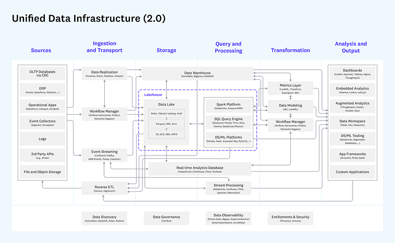
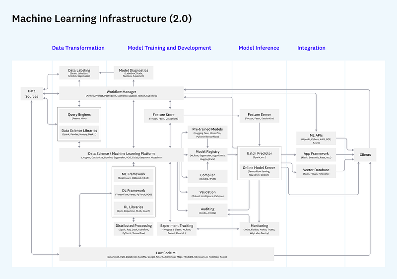
The following is a complete data infra and a complete AI/ML infra.

From the above two diagrams, we can figure out that these two groups of technical stacks are independent of each other, i.e. two silos.

Data Lakehouse

After understanding the root cause of data silos, the next question is how to solve it.

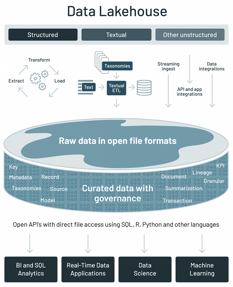
The most straightforward idea is to centralize the management of all data, which is a typical data lakehouse, and Databricks was the first to propose this idea.

In analytics scenarios, structured data is often used, while AI/ML scenarios rely heavily on unstructured data. For data lakehouses, both structured and unstructured data can be centrally managed.

In addition, data lakehouse provides a common interface for various processing engines, such as Spark and Flink for stream processing and Trino for big data querying. Thanks to the multi-engine support, data lakehouse can be applied to almost every data scenario.

Moreover, data lakehouses provide an cost and performance balance. It can support a variety of usage scenarios while at the same time saving costs. Of course, this is an advantage traded for performance.

Nevertheless, data lakehouses still don’t totally solve everything, such as the following problems.

• At the sacrifice of performance, user-facing feature still requires dedicated database support.
• Unified data storage is a challenge for privacy and compliance.
• The data is all put together and still can’t avoid the dilemma of data swamp which is the result of the data lake in the past. Although there is a catalog in the data lakehouse, it is still not transparent enough.

Most importantly, although the data lakehouse effectively mitigate the gap between data engineering and AI/ML, it is still helpless in cross public cloud scenarios.

Metadata Lake

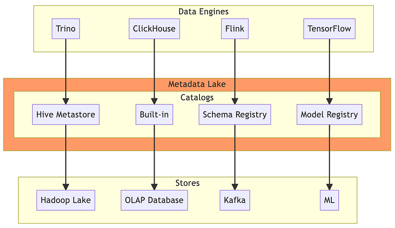
The problem we face now is the storage everywhere, and each type of storage has its own catalog, and each catalog is heterogeneous.

What if we treat the catalog as we treat the data? In other words, just as we gather all the data in one place, we gather all the catalogs in one place, so can we achieve complete governance? When we can completely govern all the data with metadata, won’t we break the data silo?

Yes, exactly. This is what the concept of metadata lake does.

From the above diagram, we can see modern data processing engines have corresponding catalogs, and Metadata Lake is designed to centralize the governance of these catalogs. In this way, there is a unified place to view all data sources and understand the internal data structure.

This concept is not new, in fact, all public clouds have launched corresponding products, like Microsoft’s OneLake and GCP’s BigLake, which are based on this concept.

However, these public cloud services can only solve the data silos within the public cloud, and there is still no solution for cross public cloud.

Fortunately, more and more enterprises have noticed this business opportunity and started to make their own products, e.g., Datastrato’s Gravitino is focused on solving the data silos across clouds.

Conclusion

We are living in a chaotic and complex era.

The amount of data is exploding, and the AI boom is exacerbating the process. In the past, we have tried to store data, clean it, transform it, and then use it. With the data we have, we’re already swamped. And with the increasing data volume, it’s only getting busier.

However, nowadays, this is not enough. We want to know what is stored and we want to be able to integrate and interact with it easily. Therefore, data governance has become an obvious subject.

That’s also why there’s an increasing number of tools geared towards metadata.

I’m also concerned about this topic because our organization recently made the transition from GCP to AWS, and governing the warehouse schema for both clouds is becoming an issue. I will leave this story for later, so let’s call it a day.

Originally published on Medium

Navigating event-driven architecture for real-time updates

Recently our engineer asked me a question.

Why do we need to periodically get the latest state via API while we design the event-driven architecture, in addition to relying on asynchronous events for data synchronization?

If we need to get the latest status periodically, then why not just synchronize the data through the API completely?

This is a good question, but before answering this question, let’s consider what our system requirements are.

Suppose we want our clients to see the latest status as much as possible, and we can only allow a maximum delay of 5 minutes.

How would we design the system to synchronize the status through events? First, we would trigger a corresponding event at the point of addition, modification, or deletion of the original data, and then synchronize the state of the original data to our system based on the event. This design ensures clients can see the latest status.

On the other hand, if we need to synchronize the raw data via the API, then we must start a periodic task, such as a crontab, every five minutes, and then periodically download all the raw data back via the API.

Both approaches meet our system needs, but the former is much lighter than the latter, until a problem occurs.

Problems of Asynchronization

The biggest problem with asynchronous events is we cannot ensure the order of the events (unless we add ordering identifiers to the event design). So it is possible that two close updates arrive in the opposite order, resulting in inconsistent data.

For example, the original data is value = A. In a short period of time, it is changed to B and then to C. However, if the order of arrival of the events is such that C arrives before B, then the client will see the result as value = B (instead of value = C).

In addition, asynchronous communication without a proper handshake process can result in event loss, which again can produce inconsistent data.

For these reasons, we often include additional mitigation via the periodic checking mentioned at the beginning. This leads to the question at the beginning, why don’t we just synchronize everything through the API?

The answer is simple, because we are comparing two completely different requirements, i.e., timeliness and accuracy.

Timeliness and accuracy are the two ends of the spectrum.

Under the fixed cost premise, we can’t ask a system to be both real-time and accurate, there must be a trade-off. Costs here include many items, such as development and maintenance costs, hardware costs, transfer costs, and so on.

When we want to achieve high timeliness, we sacrifice accuracy. But if we want to maintain a certain level of accuracy, then we move a little bit to the other end of the spectrum, i.e., periodic checking.

This is why in a distributed architecture it is better to have a BASE rather than an ACID. The E of BASE is eventual consistency, we make sure that the data will be consistent in the end, but how fast is that end? It depends on how many compromises we have to make.

Conclusion

In a software architecture, similar trade-offs occur in various scenarios.

In this case, we end up choosing timeliness over accuracy, but there may be specific scenarios where we need accuracy over timeliness, e.g., a financial reporting system.

In this case, there are two common design patterns for financial reporting systems.

• Monthly report dashboard
• Takes a while to output reports

In the first pattern, we sacrifice granularity for report presentation efficiency. On the other hand, in the latter pattern we choose to utilize additional computation time in order to achieve report accuracy. These design patterns are the result of trade-offs.

There is no one-size-fits-all solution that can be applied to all scenarios, so we need to be careful to identify the non-functional requirements behind the functional requirements when designing the architecture in order to get things right.

Originally published on Medium

Elasticsearch Index Lifecycle Management in a Nutshell

Understanding its Application Scenarios and Limitations

When we develop data-intensive applications, we usually classify data into frequently used and infrequently used, i.e. hot data and cold data. We have different ways of handling data at different “temperatures”, for example, cold data is stored in lower-cost storage, but with a lower access performance.

If the databases we use have this kind of temperature management built in, then the operation effort will be greatly reduced.

Fortunately, Elasticsearch has such a feature, called index lifecycle management (ILM).

Before we get into ILM, let’s jump to the conclusion.

There are two common ways to use Elasticsearch, one is to treat Elasticsearch as an OLTP database, just like a regular database where we CRUD each document. The scenario is we need the search capabilities provided by Elasticsearch, so each document will be a corresponding entity.

Take an e-commerce website as an example, in order to be able to search for product titles, content, etc., we will add a product as a document to Elasticsearch, and when there are any changes to the product, we will directly find out the corresponding document and modify the fields in it.

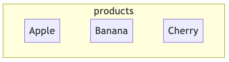
So, the modeling in Elasticsearch will be an index, let’s say products, which contains many documents representing products.

On the other hand, Elasticsearch can also be used as a time-series database. All data is continuously written to Elasticsearch, and the written documents are rarely modified. A common example of this is logs. We often use Elasticsearch’s powerful search capabilities to find specific patterns in logs. So in Elasticsearch, there may be a time-divided index, such as log-2024–04–01, log-2024–04–02 and so on.

Elasticsearch’s ILM only benefits from the latter.

ILM Concepts

Why ILM can only work on time-series data scenarios and not on OLTP scenarios?

Briefly, the unit of ILM is index, as indicated by the first letter I. Therefore, when only one index exists, there is no way for ILM to manage it. Either the whole index is hot, or the whole index is cold, and there is no way to distinguish which documents are hot and which are cold within this index.

The whole concept of ILM in Elasticsearch is to label the index with hot, warm and cold. With different labels, there will be different behaviors, for example, a cold index can only be read but not written. In addition, the nodes in the cluster are labeled so that different temperature indexes belong to specific nodes. In this way, the cold index can be placed in a lower cost machine to save cost.

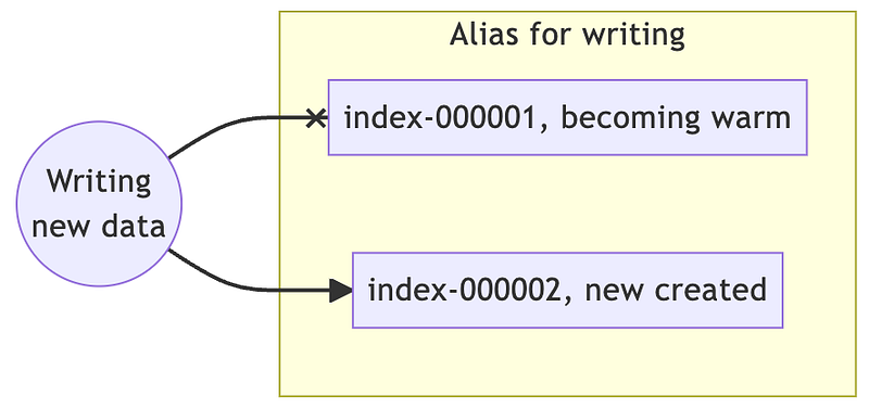
In addition to ILM, Elasticsearch has another mechanism that is often paired with ILM, which is Rollover. When time-series data is constantly written to an index, the performance of the index will inevitably degrade. Therefore, Rollover allows the index to generate a new index when certain conditions are met, and the original index will no longer accept write requests.

The principle of Rollover is to have a dedicated alias for writing to the underlying index, e.g. index-000001, and when a new index is generated, the alias is automatically switched to the new index, e.g. index-000002.

Based on the configured ILM policy, index-000001 will be converted from a hot index to a warm index, and then to a cold index, achieving a lifecycle.

This is the whole concept of data tiering in Elasticsearch.

Conclusion

Although Elasticsearch has built-in ILM, there are still many people who misunderstand the concept of ILM. The built-in ILM is indeed a very powerful capability, but it is not a silver bullet as there are limitations on the scenarios it can be applied to.

Therefore, this article mainly explains the concept of ILM and the applicable scenarios. As for the specific operation is not difficult, the official document has a detailed description, I will not dive into it.

If we want to use Elasticsearch in an OLTP scenario and want to benefit from ILM, then I think we may need to change our modeling approach so that each CRUD creates a new entity, which might be simpler in this case.

Here’s a possible approach, let’s continue with the products example.

When we add a Japanese apple at the first index, products-01.

1
2
3
4
5
6
7

POST /products-01/_doc/1  
{  
    "product_id": "0001",  
    "product_name": "Apple",  
    "description": "Made in Japan",  
    "price": 100  
}

After some time, Japanese apples were out of stock, so we switched to importing American apples. But at this time, the index has been changed to products-02 due to Rollover, and the original products-01 has been cooled down so we can’t update it.

Then we need to write the same apples and updated information in products-02.

1
2
3
4
5
6
7

POST /products-02/_doc/1  
{  
    "product_id": "0001",  
    "product_name": "Apple",  
    "description": "Made in USA",  
    "price": 50  
}

All of these indexes will have the same alias, products-search, for searching.

1
2
3
4
5
6
7
8
9
10
11
12
13
14
15
16
17

POST /_aliases  
{  
    "actions": [  
        {  
            "add": {  
                "index": "products-01",  
                "alias": "products-search"  
            }  
        },  
        {  
            "add": {  
                "index": "products-02",  
                "alias": "products-search"  
            }  
        }  
    ]  
}

Finally, we search the results directly on products-search but sort them in order, and the top one will be the final result.

1
2
3
4
5
6
7
8
9
10
11
12
13
14
15
16
17
18
19
20
21

POST /products-search/_search  
{  
    "query": {  
        "bool": {  
            "must": [  
                {  
                    "match": {  
                        "product_name": "Apple"  
                    }  
                }  
            ]  
        }  
    },  
    "sort": [  
        {  
            "_index": {  
                "order": "desc"  
            }  
        }  
    ]  
}

So the client has to de-duplicate the data using product_id, which is a case of updates. Similarly for deletions, a document labeled with a soft delete flag needs to be added so that the client can be aware that the data is invalid.

In order to implement data tiering on the backend, extra processing must be done on the client side. If the system wasn’t designed this way from the beginning, there would be a lot of development on the client side, which is not always a good approach.

Alternatively, use additional ETL to move documents that meet the criteria to a different cold index. In this way the client can maintain its existing behavior without awareness.

Anyway, there’s not much ILM can do for OLTP scenarios, it all depends on the system design.

Originally published on Medium

Making Gemini a Tarot Master

Quickly build a RAG application with Streamlit and LangChain

Nowadays, AI resources are quite available, which makes it much easier to implement RAG (retrieval-augmented generation) applications.

In order for me to keep writing programs and not to be out of sync with the technology for too long, I’m going to use LangChain to implement a Tarot bot.

I chose LangChain because it has an active ecosystem and supports multi-model design, so it’s easy to modify it according to the needs. For example, I’ll be using Gemini Pro as my LLM this time, but it’s easy to switch to ChatGPT or even the free Ollama.

The whole process is simple.

1. Crawl through the web to retrieve a lot of Tarot knowledge and examples.
2. Convert these data into vectors and write them to vector storage.
3. Build a Web App that can draw cards and present them.
4. Feed the drawn cards to AI for interpretation based on the big data.

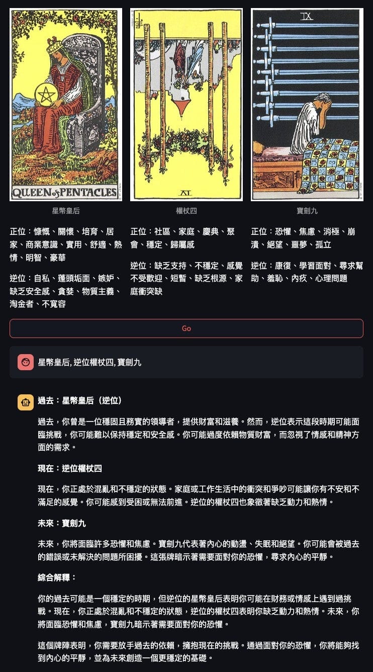
The final result will be as follows.

Apologies for the Chinese. I’ve been studying Tarot lately, so I’m more likely to get the meaning right if it is in Chinese.

This layout has a button to draw cards. When the button is pressed, three cards are turned over, each with an upright meaning and a reversed meaning. Finally Gemini will try to give a full explanation of the meaning of each card in context.

Let’s get our hands dirty.

Preconditions

Let’s start by installing the packages that will be used.

pip install langchain-google-genai langchain pymongo

Implementing a web crawler

Since web crawlers are not the focus of this article, and web crawlers involve finding targets and parsing web content, let me get directly to the heart of the RAG problem.

How to put the material into vector storage?

First, we make a basic declaration about which data store we want to use and what kind of embedding we want to use to convert the text into vectors.

In this example, I’ve chosen to use MongoDB Atlas, so let’s get the settings right.

1
2
3
4
5
6
7
8

from pymongo import MongoClient  
  
# MONGODB_ATLAS_CLUSTER_URI will contain credentials, please modify it accordingly.  
client = MongoClient(MONGODB_ATLAS_CLUSTER_URI)  
DB_NAME = "langchain_db"  
COLLECTION_NAME = "test"  
ATLAS_VECTOR_SEARCH_INDEX_NAME = "index_name"  
MONGODB_COLLECTION = client[DB_NAME][COLLECTION_NAME]

Next is Gemini’s own embedding.

1
2
3
4
5
6

import os  
from langchain_google_genai import GoogleGenerativeAIEmbeddings  
  
# GEMINI_PRO_API_TOKEN is a credential, please modify it accordingly.  
os.environ["GOOGLE_API_KEY"] = GEMINI_PRO_API_TOKEN  
embeddings = GoogleGenerativeAIEmbeddings(model="models/embedding-001")

Before writing to storage, the data needs to be pre-processed. Assuming all the data is in JSON format, we need to split the JSON into smaller chunks to make it easier to use.

1
2
3
4
5
6
7

from langchain_text_splitters import RecursiveJsonSplitter  
  
splitter = RecursiveJsonSplitter(max_chunk_size=300)  
# json_data is the data source in JSON format  
json_chunks = splitter.split_json(json_data=json_data)  
# docs will be stored  
docs = splitter.create_documents(texts=[json_data])

Once everything is ready, it’s just time to convert the data into vectors and write them to MongoDB.

1
2
3
4
5
6
7
8
9

from langchain_community.vectorstores import MongoDBAtlasVectorSearch  
  
# insert the documents in MongoDB Atlas with their embedding  
vector_orig = MongoDBAtlasVectorSearch.from_documents(  
    documents=docs,  
    embedding=embeddings,  
    collection=MONGODB_COLLECTION,  
    index_name=ATLAS_VECTOR_SEARCH_INDEX_NAME,  
)

Depending on the state of the crawler and the results, this stage can take a lot of time, both for retrieving data and for writing to storage.

Web App implementation

It’s not difficult to build a Web App quickly, as I’ve introduced in my previous article about Streamlit.

Therefore, I will only talk about two key points this time.

There are many spreads in Tarot, each spread has different layouts and corresponding Gemini prompts, so we need to prepare a detailed explanation of the spreads for Gemini to know how to interpret them.

1
2
3
4
5
6
7

if spread_type == 'Time Flow':  
    spread = init_time_flow_spread()  
    sys_prompt = '''  
This is a Time Flow Tarot spread where three cards are drawn to represent the past, present and future.  
  
Based on the user's question, the meaning of the three cards drawn by the user, and the following {context}, a reasonable explanation is given.  
    '''

The tarot cards are drawn in upright and reversed positions, so we can’t just use the file paths in st.image, we need to read out the files and process them and use numpy.ndarray as the parameter.

1
2
3
4
5
6
7
8
9

def open_image(fp):  
    from PIL import Image  
    import numpy as np  
  
    image = Image.open(fp)  
    image_array = np.array(image)  
    flipped_image = image.transpose(Image.ROTATE_180)  
    flipped_image_array = np.array(flipped_image)  
    return image_array, flipped_image_array

Integrate with Gemini Pro

For Gemini to learn about Tarot, the results of the previous crawler are required, so the first step is to make Gemini able to retrieve the vectors we have stored, i.e. the R of the RAG.

We’ll use the mentioned embedding and the MongoDB settings.

1
2
3
4
5
6
7

vector_search = MongoDBAtlasVectorSearch.from_connection_string(  
    MONGODB_ATLAS_CLUSTER_URI,  
    DB_NAME + "." + COLLECTION_NAME,  
    embeddings,  
    index_name=ATLAS_VECTOR_SEARCH_INDEX_NAME,  
)  
retriever = vector_search.as_retriever()

Next we need to build the LLM using Gemini Pro.

1
2
3

from langchain_google_genai import ChatGoogleGenerativeAI  
  
llm = ChatGoogleGenerativeAI(model="gemini-pro", convert_system_message_to_human=True)

Finally, the whole chain is connected.

1
2
3
4
5
6
7
8
9
10
11

from langchain.chains.combine_documents import create_stuff_documents_chain  
from langchain.chains import create_retrieval_chain  
from langchain_core.prompts import ChatPromptTemplate  
  
# sys_promopt is based on Tarot's Spreads.  
prompt = ChatPromptTemplate.from_messages([  
    ('system', sys_prompt),  
    ('user', 'Question: {input}'),  
])  
document_chain = create_stuff_documents_chain(llm, prompt)  
retrieval_chain = create_retrieval_chain(retriever, document_chain)

With the whole chain, we can ask Gemini to start his show.

1
2
3
4
5

# input_text is the three cards drawn by the user.  
response = retrieval_chain.invoke({  
    'input': input_text,  
    'context': []  
})

Conclusion

This is the simplest example of a RAG implementation, applying all RAG elements, and each piece can actually be modified as needed. The domain knowledge of application is the results from crawlers, and this application just uses the information to answer questions.

At the moment, I don’t intend Gemini to act like a real soothsayer with the user. Instead, Gemini will provide a one-time recommendation. For me, Tarot is a tool for inner dialogue, not for seeking magic.

The whole project is on Github.

Although this application has both UI and AI integration, the total number of code lines is only 150. I have to say, both Streamlit and LangChain are really great at packaging complex implementations in abstract and sophisticated interfaces, so that users can easily write functionality instead of dealing with miscellaneous things.

Here are some of the LangChain materials I have references to.

• gemini-pro: https://python.langchain.com/docs/integrations/chat/google_generative_ai
• gemini-embedding: https://python.langchain.com/docs/integrations/text_embedding/google_generative_ai
• mongo-atlas-vector: https://python.langchain.com/docs/integrations/vectorstores/mongodb_atlas
• json-splitter: https://python.langchain.com/docs/modules/data_connection/document_transformers/recursive_json_splitter

Originally published on Medium

Experience a boost in API response times with our paradigm-shifting move from Semi-Lambda to TiDB & Kappa architecture

We recently launched a big technical revamp, and the results have been impressive. We’ve seen a 9x improvement in response times for specific APIs (from 9 seconds down to 1 second).

You may ask why the API response time is so long. It’s mainly because of the product characteristics, it’s a data product, there will be a lot of data aggregation and analysis, and the API response will be the result of a period of analysis. Therefore, in general, there will be a longer latency.

Nevertheless, through this technical revamp, we have significantly reduced the API latency while maintaining the product features.

This is due to two core changes.

1. Database changes
2. Kappa architecture

Let’s take a closer look at what we did.

Semi-Lambda Architecture

At first, our architecture is a “semi-Lambda” architecture. To understand what a semi-Lambda architecture is, let’s first look at a Lambda architecture.

A typical Lambda architecture has three components.

1. Batch layer
2. Speed layer
3. Serving layer

Data processing from the data source is divided into two paths, one is periodic batch processing, which has the advantage of processing a large amount of data quickly.

On the other hand, in order to enhance the freshness of the analysis, there is real-time processing to calculate the data in the current time period. The results from both sides are aggregated into a serving layer so that end users can get the final results.

For example, if the time is 12:30 and the batch layer runs every full hour, then the data from 12:01 to 12:30 will be processed by the speed layer.

The above is a standard Lambda architecture.

Then, what is a semi-Lambda architecture? The illustration is as follows.

We also have a batch layer and a serving layer, but we are missing the speed layer. Instead, we write the raw data directly into the serving layer, and the client, e.g. API, which is invoked by the upper layer, runs the logic to process the raw data and combine it with the batch result.

In other words, we are the on-the-fly speed layer.

The drawbacks of such an architecture are obvious.

1. Postgres is a monolithic database, so even though it can be read-write split, the replicas still need to synchronize with the master constantly. This is fatal in large raw data write scenarios, where I/O consumes a lot of system resources.
2. Postgres is limited in its capability to handle big data. Although it is possible to make data blocks smaller and easier to read by partitioning, a single database is not enough when the algorithm is designed for a large number of partitions.

Therefore, we need to propose solutions to these two problems.

Streaming ingest problem

First of all, we need to solve the database bottleneck of writing large amounts of data. Therefore, a proper database is essential.

For those who have been following me, you should know I have been studying RTOLAP databases such as Apache Pinot for some time. But in the end, we didn’t go with RTOLAP.

The main reason is RTOLAP database does not perform well in two specific scenarios.

1. Upsert
2. Join

Because of the application features, we need to perform frequent upserts on big data, and in addition, we need to do a large number of joins, doesn’t matter if it’s a cross-table join or self-table join.

On the other hand, it is difficult to say RTOLAP database has comprehensive support for SQL statements, and we want to minimize the amount of trial-and-error work required for migration, so we didn’t choose RTOLAP database in the end.

Fortunately, around the same time, we got some help from a vendor and learned about a distributed database completely compatible with MySQL, i.e. TiDB. Previously, I wrote an article describing TiDB application scenarios. In fact, TiDB can support both OLTP and OLAP scenarios, fitting our needs.

Speed layer problem

Once the database selection is finalized, the next step is to address the lack of a complete speed layer.

There are two possible directions.

1. Build a complete Lambda speed layer.
2. Change to Kappa architecture

In the end, we chose the latter and started to move the architecture to Kappa.

The reason is both Lambda and Kappa need to build streaming processing capabilities, but to build a speed layer for the Lambda architecture we still need to rewrite the batch logic in a streaming framework. It would be better to migrate the batch logic to the Kappa framework so that if there is a need for any feature in the future, we just need to add the new logic to the streaming framework.

This is one of the advantages of Kappa over Lambda, there is no need to maintain two pipelines (batch and real-time) with the same logic.

After moving to the Kappa paradigm, you can see that the whole architecture has become simple, with Flink being responsible for data processing and batch processing disappearing. In addition, Postgres was moved to TiDB, which of course required changes to the query syntax, but it was well worth it.

Finally, we solved the OLAP query latency problem by using streaming pre-processing and the power of the TiDB distributed database.

Conclusion

Paradigm shift is a battle against time, and how to keep optimizing the system while guaranteeing development productivity is a big challenge.

In addition to initiating discussions and a series of technical selections, it is more important to plan the actual migration and develop efficiently. This requires architects, PMs, and developers to work together.

The question is frequently asked: How much of a benefit is this migration? It’s a tough question to answer before getting one’s hands dirty. But if we don’t know the benefits, how can we have the confidence to invest for such a long period of time?

From my point of view, we need to list the problems we want to solve and prioritize them in a way that will affect the final solution. Then, identify one or two showcases to act as pilots, and learn as much as possible from these showcases, rather than launching a large-scale revamp all at once.

When results are achieved in the showcases, we will be able to measure the benefits.

Engineering is different from science in nature. Engineering is learning by doing, not by theorizing. Airplanes fly before scientific theories can explain them, that’s my mindset on technical revamping, let’s see what you guys think too.

Stackademic 🎓

Thank you for reading until the end. Before you go:

• Please consider clapping and following the writer! 👏
• Follow us X | LinkedIn | YouTube | Discord
• Visit our other platforms: In Plain English | CoFeed | Venture | Cubed
• More content at Stackademic.com

Originally published on Medium

Simplify Web App Development: Code Lite, Create Big!

Empower your ideas with Streamlit’s Magic — build feature-rich Web Apps effortlessly

Hello data engineers and backend engineers!

• Have you ever wanted to implement a Web App but didn’t know where to start because you don’t have frontend skills?
• Have you ever struggled to write interactive components and spent a lot of development time?
• Have you ever wanted to present an idea quickly but didn’t have the right tools?

Here’s your savior, let’s welcome Streamlit.

It’s a full-stack framework for Python that allows you to write scripts to generate a Web App that can really work, and it supports a variety of interactive components as well.

Let me show the power of Streamlit with a real-world example.

The above Web App is a demo of what I actually developed after I know about Streamlit, with several interactive components and integration with the database, and it’s even already live. Guess how long it took me?

Less than an hour.

A beginner who can write Python can write a Web App in a very short time, and I have to say that this practical experience is truly amazing.

Moreover, the goal of Streamlit is to provide a framework for fast data visualization, so even drawing is as easy as the following.

In the Streamlit gallery there are a lot of examples that have already been done, and you can see that Streamlit covers almost all of the common components needed for daily work.

Demo Site

Let’s go back to the beginning of the example I worked on.

As we can see from the diagram, we have used six input components in the following order.

• Select box
• Calendar
• Time picker
• Text input
• Number input
• Button

The actual code is quite simple.

1
2
3
4
5
6
7
8
9
10
11
12
13
14
15
16
17
18

@st.cache_data(ttl=600)  
def get_user():  
    db = client.dev  
    users = db.user.find().sort('_id', -1)  
    users = [x['name'] for x in users]  
    return users  
  
user = st.selectbox('User', get_user())  
d = st.date_input('Date')  
t = st.time_input('Time')  
item = st.text_input('Item')  
amount = int(st.number_input('Amount', step=1))  
dt = datetime.combine(d, t)  
  
if st.button('Submit') and item and amount:  
    db = client.dev  
    db.accounting.insert_one({'DateTime': dt, 'Item': item, 'Amount': amount, 'User': user})  
    st.write('Submitted')

Each input component is actually a function, and the return value is the result of the input component, which makes the whole program as easy as writing a script. There is no callback and no signal, which makes the development of Web App extremely trivial.

After the script is executed, the corresponding frontend page will be generated.

Why am I so impressed?

For someone without frontend skills, making an interactive UI used to rely on packages like PyQt or tkinter.

Taking PyQt as an example, the way to write a select box is as follows.

1
2
3
4
5
6
7

def show():  
    text = box.currentText()  
    print(text)  
  
box = QtWidgets.QComboBox(form)  
box.addItems(['A','B','C','D'])  
box.currentIndexChanged.connect(show)

For components to be able to interact, they need to deal with event binding in addition to appearance definition, which is not intuitive.

Each component has its own events, and various callbacks need to be defined, all of which are learning curve. In fact, tkinter is a similar implementation.

But in Streamlit, you can do the same thing with just one line.

1
2

text = st.selectbox('Label', ['A','B','C','D'])  
print(text)

This makes development very natural. I call the component I need, and the return result is what I want.

Conclusion

The greatest advantage of Streamlit is that a person without any frontend skills (HTML, CSS and Javascript) can build a full-featured Web App in a very short time. In addition, Streamlit is a differentiator from many UI packages in providing a simple concept that makes the operation of interactive components natural, and truly what you see is what you get.

Streamlit is best suited as an internal data analytics platform or a PoC for quick validation, while its biggest shortcoming is that such a Web App is not well suited for high-traffic systems.

The main reason is because Streamlit, in order to build up the simple concept mentioned above, its implementation is to reload the whole script every time any component changes, which has a very high system load.

On the other hand, this means that the Web App is stateful and cannot be scaled horizontally through a load balancer.

And Streamlit itself so far does not support Gunicorn, so its vertical scalability is limited.

In summary, Streamlit is best suited for Data Apps, as mentioned in the official website.

A faster way to build and share data apps.

Nevertheless, for me, even though I’m able to develop frontend pages, I don’t feel I’ll ever touch HTML again. After all, who wants to deal with the extra technical stack when you can do it all in Python.

Stackademic 🎓

Thank you for reading until the end. Before you go:

• Please consider clapping and following the writer! 👏
• Follow us X | LinkedIn | YouTube | Discord
• Visit our other platforms: In Plain English | CoFeed | Venture | Cubed
• More content at Stackademic.com

Originally published on Medium