CT Wu

Hands-On WrenAI Review: Text-to-SQL Powered by RAG

Deep dive into customization, performance, and practical insights for seamless SQL generation

WrenAI is a text to sql solution that I’ve been following for a while. Recently, I have some time to try it out, so let me share my experience.

First of all, according to the installation guide provided by the official document, we can generally deploy WrenAI to the local machine. As for the integration with local Ollama, there are some sample configuration files that can be used.

However, there are still some details to be adjusted that are not mentioned in the document. For example, if we use the ollama/nomic-embed-text mentioned in the document as the embedder, then we need to change the embedding_model_dim of the configuration file from 3072 to 768, which is a detail that can be easily overlooked.

Just provide the appropriate settings and WrenAI will work fine.

By the way, I am using MySQL and the official MySQL test dataset.

WrenAI Advantage

In addition to schema-based chat Q&A, WrenAI has another awesome feature.

It provides the flexibility to customize prompts, and under WrenAI’s Knowledge page, it is possible to enter pre-designed questions and corresponding SQL answers. In addition, we can also enter additional commands to provide the AI with additional “parameters”.

After I disassembled WrenAI’s prompt, I realized that these Knowledge play a very important role in determining the final SQL’s appearance. This customization provides a reliable fine tuning opportunity when integrating a usage-based data source like BigQuery.

WrenAI Disadvantage

This is a fairly new project (0.19.2 at the moment), so there are bound to be some bugs.

I’ve encountered two problems that I find quite annoying.

First, when I first logged in the homepage, WrenAI will provide some recommended questions based on the data model, so that users can get into the situation quickly. However, this kind of full model scanning consumes a lot of computing power, and if the model is not strong enough, basically we cannot get the result.

It doesn’t matter if we can’t get the recommended questions, but WrenAI’s error handle is not well designed, it will provide a lot of unimportant built-in questions, and there is no align project setting for the language. I’ve mentioned a GitHub issue about this.

Secondly, even though there are not many data models in the source and not many columns, the llama3.1:8b model still has a certain percentage of AI hallucination.

Since I’m a data engineer, it’s easy for me to read SQL, so it’s easy for me to find the problem, and WrenAI also provides a good correction mechanism to correct the original answer, so I haven’t encountered too many obstacles in using it.

However, I am worried that people who are not familiar with datasets and SQL may have unexpected surprises if they use it directly.

Lastly, and this is both a strength and a weakness of WrenAI, WrenAI is based on a RAG implementation to generate SQL, which requires a strong model to support. Take my llama3.1:8b running on MacBook Pro M2, a simple problem (joining a few tables) would take more than 5 minutes, not to mention the complicated problems, and it’s common to run into internal server error.

I won’t go into the details of some minor Web UI issues and design flaws in the interaction with the backend.

Wrap Up

WrenAI uses RAG as the foundation to implement a pretty good text to sql solution, and because it is based on RAG, there is a lot of flexibility to customize the prompt.

However, because it is a RAG, the computing power and model capacity are high, and the effect on small model scenes needs to be strengthened.

I will do more experiments with more powerful models and expect to get better results. Overall, WrenAI is a product worth trying.

Originally published on Medium

MCP Make Me Happy

Empowering productivity with integrated AI tools

Recently, the topic of MCP has suddenly become extremely popular, and I guess the main reason is there are a lot of MCP servers in the eco-system.

In order to increase productivity, I’ve spent some time to test some MCP combinations. After all, computer resources are limited and I can’t use all MCPs at once, so I’ve picked a few that I find most useful.

I usually use the Smithery MCP registry, which has a large number of projects posted. Here are my favorite combinations.

• Sequential Thinking
• Desktop Commander
• Duckduckgo Search

First of all, sequential thinking I believe is the core, even though nowadays AI models usually have CoT, it is still necessary to ask AI to disassemble the workflow through prompt. By disassembling the workflow, the AI will be able to correctly invoke the corresponding tools to solve the problem. So sequential thinking plays the role of the brain.

Next, the desktop commander is the body that does all the work. Because the desktop commander can read files, write files, and execute commands, it can do everything a command line can do.

Finally, there is duckduckgo search, which provides additional information to accomplish specific tasks. I have to say this is not really used very often, but if we need to find the most recent information, a web search can be helpful.

Demo

This project is a weather prediction program I built to explain machine learning to team members. It took less than 10 minutes to complete without opening an IDE or writing a single line of code.

https://github.com/wirelessr/scikilearn-demo

The Claude Desktop and the three MCPs mentioned above were used.

System instruction: You are a professional ML developer who is familiar with various python ML frameworks and is able to call on various tools to actually operate the computer, e.g. read files, write files and execute commands.

We start by setting up the roles and game rules for the AI, and then we actually move on to development.

Help me create a scikit-learn demo project on my desktop to predict temperature, need to have test data. Also, this project needs to have a virtual env that does not pollute my system python.

At this point Claude will start building a draft of the project, but he has not separated train from predict and has not yet trained the model. Therefore, let’s ask the AI to modify the project and actually build the model.

Is this script already trained? How can I use it to predict tomorrow’s temperature? Run the commands directly to build the model.

Claude then creates the python environment via virtual env and installs the dependencies via pip. Once the environment is set up, Claude actually runs python src/train.py to train the model.

Go to the Internet and look up today’s weather information and use this project to predict tomorrow’s weather.

This is where duckduckgo comes in and looks up the required parameters, such as today’s temperature and humidity, and runs python src/predict.py to provide the final result.

At this point, the project is completed, but for ML teaching is not enough, so I then asked Claude to write a clear description and comments.

This is a tutorial project and I need README.md and good comments.

In the end, the project is what you see on Github. I didn’t write a single line of code and I didn’t use an IDE, but the project is complete.

Originally published on Medium

Evolution of RAG: Baseline RAG, GraphRAG, and KAG

Enhancing LLM accuracy with structured knowledge, inverted indexes, and dynamic retrieval

This article focuses on the evolution of RAG, so technical details will be skipped to avoid this article being too geeky.

Using LLM for chatbot is the most common application nowadays, but the answer of LLM is too generalized to serve specific application scenarios.

Therefore, Retrieval-Augmented Generation, aka RAG, has been developed.

Simply put, it is to store the specialization data needed by LLM, so that LLM can refer to it when answering.

Baseline RAG

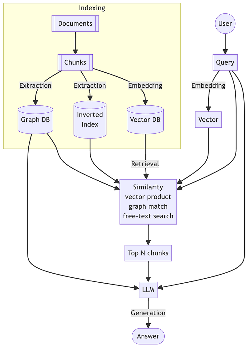
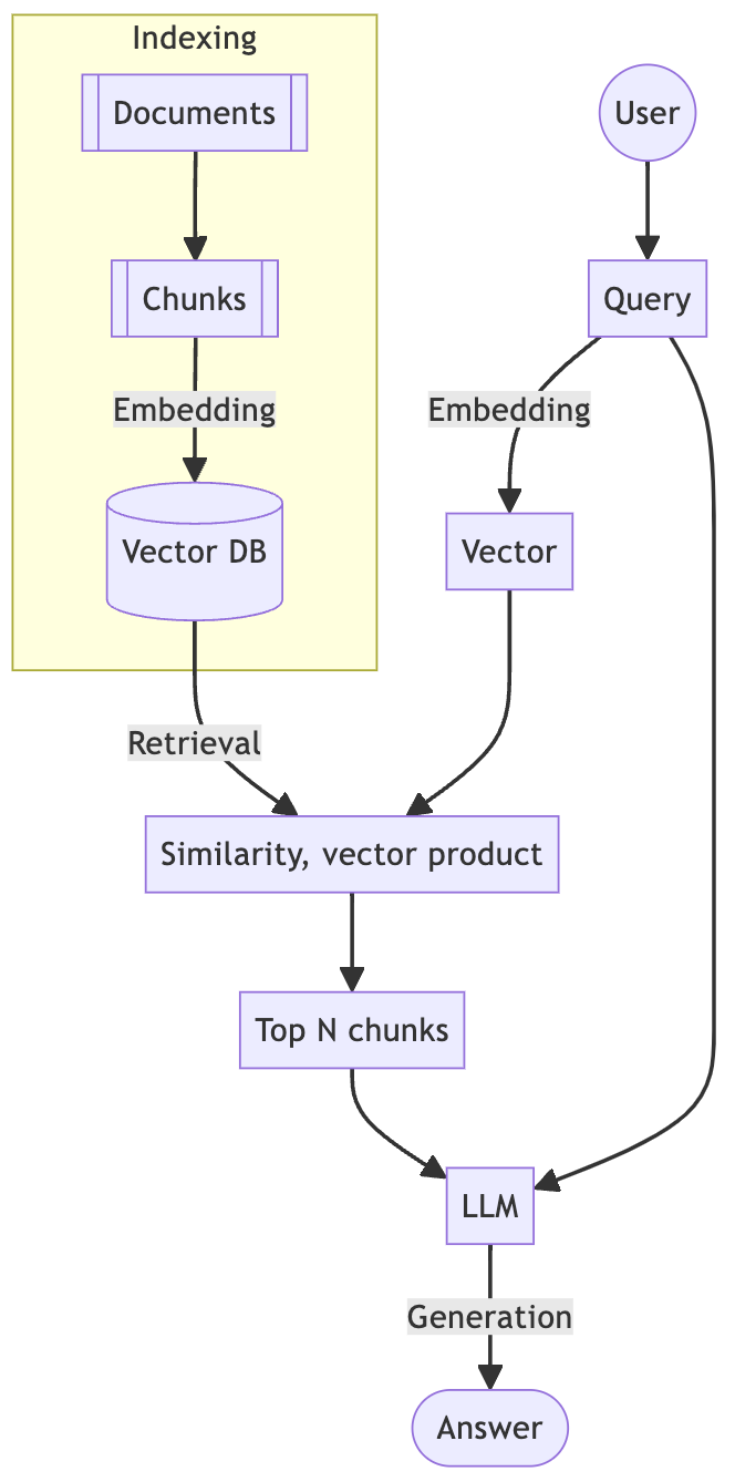
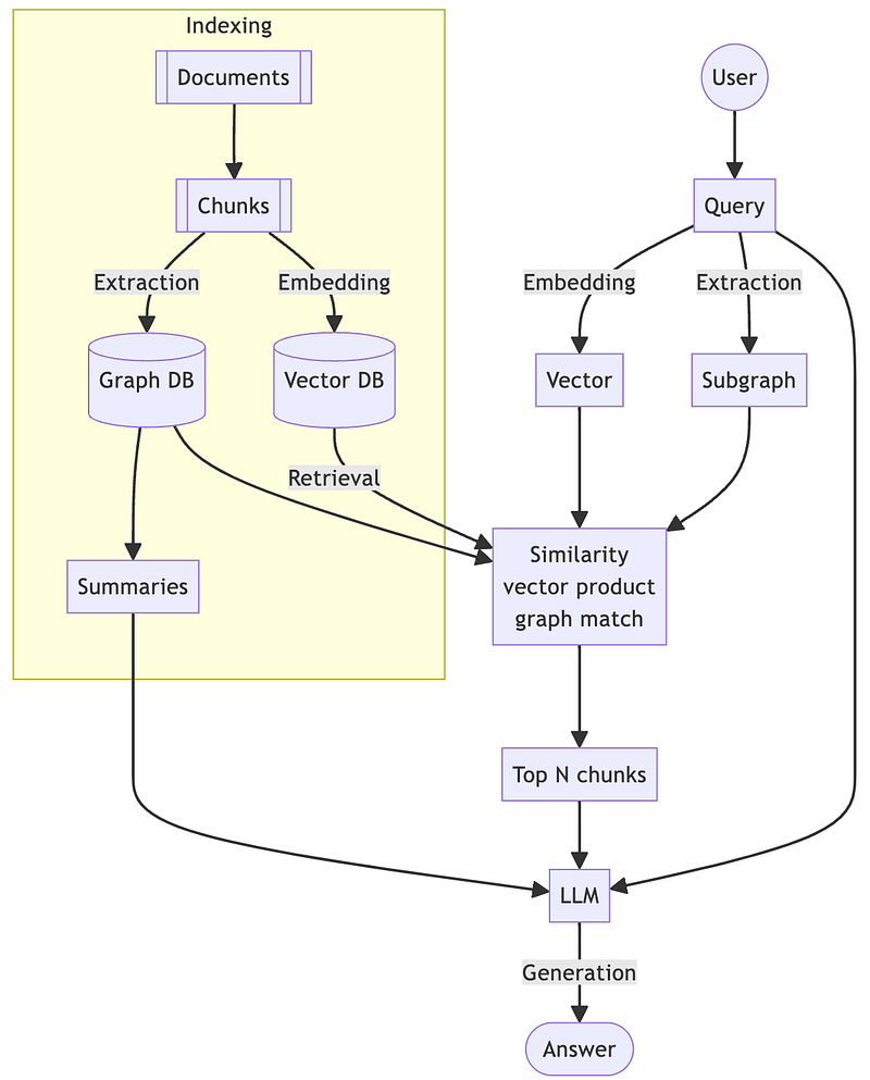
A traditional RAG process is as follows.

Indexing in the left side means to process the data that LLM needs to refer to in advance, and the processing flow is to first divide the chunks and then vectorize the chunks into the vector database.

When the user asks a question, he also needs to vectorize the query and take the first few similar results from the vector database, which is usually the order of vector product. These chunks are fed to the LLM along with the query, and the LLM generates a “good” answer.

From the above flow, it is obvious that traditional RAG encounters several problems.

1. Context fragmentation due to chunks.
2. Vector product is too simple, losing reasoning ability.
3. Vectors do not have verification capability, so it is easily to answer the wrong question.

In order to improve the reasoning ability and overcome the problem, GraphRAG was born.

GraphRAG

To avoid getting into too much in depth theory, let’s look directly at the process.

From the diagram, we can see that GraphRAG has more Graph support (as the name suggests) than traditional RAG.

In particular, this Graph consists of these three elements.

• Entity
• Relationship
• Statement description

The following is an example.

• (OpenAI) –[developed]–> (ChatGPT)
• (ChatGPT) –[is a]–> (LLM)
• (ChatGPT) –[published in]–> (2022)
• (ChatGPT) –[uses]–> (Transformer)
• (Transformer) –[is a]–> (deep learning architecture)
• (Transformer) –[published in]–> (2017)
• (Transformer) –[is developed by]–> (Google)

By extracting key information from chunks and constructing a Knowledge Graph, aka KG, the process is similar to the human brain.

For example, the hippocampus converts short-term memories into long-term memories by filtering and translating information, so that it can use these memories to get better ideas when it encounters similar situations in the future.

These KGs are graphs, which are not always easy for LLM to use, so there is another important process in GraphRAG called summarization, where these KGs are summarized into paragraph and paragraph of text.

With summarization, LLM can have a more full picture and get a relatively accurate answer.

Nevertheless, GraphRAG has its shortcomings.

1. Summaries and KGs can be helpful, but they also have the potential to diffuse specialized knowledge.
2. Although summarization can help to expand context, the reasoning ability is still insufficient.
3. The noise introduced by summarization can still create hallucination.

Therefore, the idea of converting from KG to summarization is not feasible. However, KG itself is a valuable design, as it simulates the process of knowledge generation.

What if we could make AI work more like the human brain? Therefore, we meet the Knowledge Augmented Generation, also known as KAG.

KAG

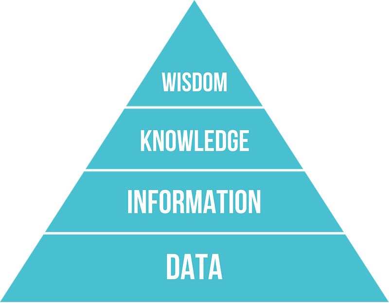
The DIKW pyramid is a famous model that describes the process of wisdom concentration, and it is what we are trying to do to make RAG accurate.

So, in the GraphRAG implementation, we filter Information from Data, and then try to build a Knowledge Graph. However, the human brain does not think in one direction, any wisdom is generated with multiple references.

The KAG paper introduces a lot of complex theories, but in short, KAG tries to allow KG to connect back to the original chunk and add more semantic references to the query rather than just vector references, which results in a significant improvement in domain-specific knowledge.

In terms of process, KAG adds inverted indexing and full-text search, so it can be more semantically precise. In addition, the extracted KG will become the source of input for LLM, so that LLM can have a more comprehensive knowledge base.

In GraphRAG, only those summaries are provided to LLM, but KAG does not do summaries, but submits the complete KG together with original text to LLM.

The ability to accept such a large number of inputs is also due to recent modeling advances, such as Gemini 2.0 Flash.

KAG has a lot of in-depth technical tuning, which makes it difficult to fully implement. However, just adding KG and full text searching over traditional RAG will already achieve good results, and it’s not too difficult to do both, which is the core value of KAG.

Wrap Up

Making LLM accurate is a difficult task, especially if we want to turn LLM into a commercial product, it is even more important to answer the question correctly.

Traditional RAGs have limited ways to improve the accuracy of LLMs, only chunking, embedding and prompting, and then adding rerank and other mechanisms to allow the Top N to find better results.

GraphRAG adds the concepts of KG and summarization to the traditional RAG to extend the context.

KAG, on the other hand, is based on GraphRAG and adds KG’s bi-directional links and inverted indexes.

All of these techniques are designed to expand the contextual information when LLM generates answers, and gradually enable LLM to be accurate enough in specific scenarios.

In fact, there are some additional variants, such as Corrective RAG aka CRAG. However, this kind of variants do not directly enhance the thinking ability of LLM, but rather assist LLM through some external mechanism, so I did not include them.

In summary, the evolutions of RAG are as follows.

LLM -> RAG -> GraphRAG -> KAG

RAG is a concept that has only been around for two years, and it’s exciting to see how quickly it has evolved.

Originally published on Medium

Integrating project management and technical trade-offs for agile system evolution

Recently, I have had some insights about microservice decomposition.

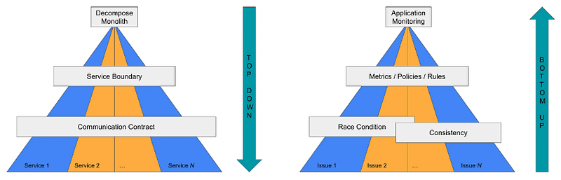
In the past, when discussing microservices decomposition, we usually start from the technical perspective, identify the domain boundary and then cut into the problem from the technical perspective to find out the appropriate decomposition solution.

The book Monolith to Microservices describes a number of technical “patterns” that cover most of the scenarios at a high level.

In general, there are three approaches:

1. Split the database first, then the code
2. Split the code first, then the database
3. Split them both at once

However, the third approach is highly discouraged in the book, and in my personal experience as well.

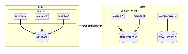
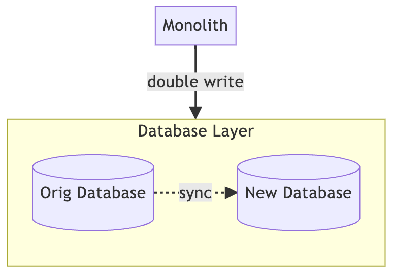
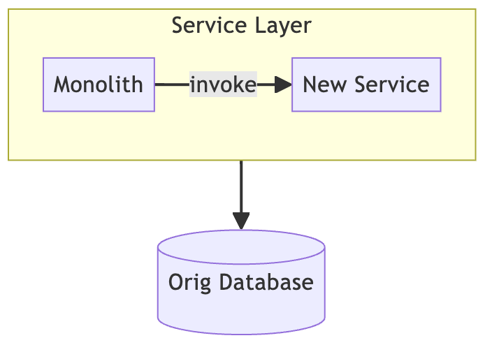
For example, in the following diagram, when we want to separate module C into a microservice, two new components are created, microservice C and a new database.

Under the first approach, we would have the monolith begin to double-write the two databases and try to make the two databases consistent.

Once we can ensure that the data is consistent, we will start to develop Microservice C and then transfer some functions from the monolith to the new service.

On the other hand, in the second approach, we will start implementing Microservice C directly, but the new service will still use the original database.

When the new service is developed and the functionality of the monolith is transferred to the new service, then we will start to handle the database split.

There is a lot of technical selection in the book about which approach to take, and there are advantages and disadvantages to both approaches. Therefore, I highly recommend that book, and I believe that anyone who needs to implement a microservice decomposition needs to read it.

Nevertheless, I want to approach this issue from a different perspective.

Team Topology Matters

The choice should be based on team topology and project planning.

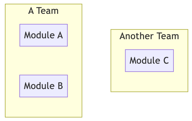
If the team topology follows Conway’s Law, i.e., Module C or Microservice C is governed by an independent team, then the second approach is much better.

The main reason is dealing with database split in the first place will face a lot of real-world challenges, which will inevitably slow down the project tempo and lengthen the development cycle.

When a system is no down time, it means a continuous write request, and how to keep the database consistent and up-to-date in such a scenario is a difficult problem.

There are many solutions, but none of them are silver bullets, and all of them need to be designed for a specific scenario.

For example,

1. Use a strong consistency-guaranteed solution such as 2PC or XA. In practice, this is seldom used, because of the performance loss and the limitations.
2. Double-write on the write side with continuous compensation. This is because the application’s double-write cannot be guaranteed to be completely consistent, and may be partially successful and partially failure due to an exception or scaling, so a compensation mechanism is needed to correct this on a regular basis.
3. Use outbox pattern or event driven. By converting all write requests into events and ensuring event process is idempotent, we can ensure all databases are updated correctly. However, this is a huge change, and the real-time nature of the writes will be degraded.

The above three solutions are common, but they all have their limitations, and the amount of development is extremely large. Moreover, in order not to affect the data structure, we usually suspend the feature iteration until the database split is finished.

And that’s not the worst part. The database split is not the end of the story because it still takes time to develop the new service and the original monolith needs time to migrate the functionality.

In other words, when we do a database split, it will affect the project’s progress, and for a long time.

So what are the benefits of splitting the code first?

First of all, when the new service exposes the interfaces, the old monolith will be able to migrate functionality based on these new interfaces. Once the migration is complete, the old monolith can start running subsequent feature iterations without having to wait for the database split.

The impact of the database split is therefore limited to the microservices team and does not extend to other teams.

Conclusion

Decomposing microservices in a monolith is always a tough challenge.

Because there is no one-size-fits-all solution, most of them need to be customized based on the scenarios. The only way to become an expert in decomposing microservices is to experience more scenarios.

Most books only look at this matter from a technical point of view, but as I gain more and more experience, I realize that the technical aspect of decomposing microservices only takes up a small part of the picture, and it’s more about compromises and trade-offs between various realities.

I’m trying to approach this topic from a project management perspective because I’ve had the experience.

Originally published on Medium

Benchmarking Lakehouse with TPC-DS

A step-by-step guide to importing TPC-DS data into Apache Iceberg

Apache Iceberg is already a popular lakehouse format that is supported by many query engines. What should we do if we want to make a technical selection among many query engines?

In the data warehouse domain, the most commonly used standard is TPC-DS, which defines several common scenarios and provides a set of standardized queries. Generally speaking, TPC-DS is the gold standard for benchmarking performance.

Although TPC-DS is quite popular and there are many common connectors for dumping test data into various databases, and even Trino, a pure computing engine, provides a dedicated catalog for TPC-DS, there is no such thing as a TPC-DS for lakehouse at the moment.

Lakehouse does not have a good connector for this purpose. Therefore, in this article we will try to describe how to dump the test data of TPC-DS into Iceberg’s lakehouse.

Experiment environment setup

Regarding how to build the TPC-DS tools is not the focus of this article, so I’ll start by assuming that dsdgen is already installed.

First, let’s generate a test data package.

1

dsdgen -SCALE 1 -DIR /home/ec2-user/sample

Once we have the test data, we need to build the Iceberg environment and import the data.

Although I’ve provided some Iceberg playgrounds before, this time I’d like to use tabular’s experiment environment. The main reason is that the tabular environment also includes a spark notebook, which helps a lot.

1
2
3
4
5
6
7
8
9
10
11
12
13
14
15
16
17
18
19
20
21
22
23
24
25
26
27
28
29
30
31
32
33
34
35
36
37
38
39
40
41
42
43
44
45
46
47
48
49
50
51
52
53
54
55
56
57
58
59
60
61
62
63
64
65
66
67
68
69
70
71
72
73
74
75

services:  
  spark-iceberg:  
    image: tabulario/spark-iceberg  
    container_name: spark-iceberg  
    build: spark/  
    networks:  
      iceberg_net:  
    depends_on:  
      - rest  
      - minio  
    volumes:  
      - ./warehouse:/home/iceberg/warehouse  
      - ./notebooks:/home/iceberg/notebooks/notebooks  
      - ./sample:/home/iceberg/sample  
    environment:  
      - AWS_ACCESS_KEY_ID=admin  
      - AWS_SECRET_ACCESS_KEY=password  
      - AWS_REGION=us-east-1  
    ports:  
      - 8888:8888  
      - 8080:8080  
      - 10000:10000  
      - 10001:10001  
  rest:  
    image: tabulario/iceberg-rest  
    container_name: iceberg-rest  
    networks:  
      iceberg_net:  
        aliases:  
          - iceberg-rest.minio  
    ports:  
      - 8181:8181  
    environment:  
      - AWS_ACCESS_KEY_ID=admin  
      - AWS_SECRET_ACCESS_KEY=password  
      - AWS_REGION=us-east-1  
      - CATALOG_WAREHOUSE=s3://warehouse/  
      - CATALOG_IO__IMPL=org.apache.iceberg.aws.s3.S3FileIO  
      - CATALOG_S3_ENDPOINT=http://minio:9000  
  minio:  
    image: minio/minio  
    container_name: minio  
    environment:  
      - MINIO_ROOT_USER=admin  
      - MINIO_ROOT_PASSWORD=password  
      - MINIO_DOMAIN=minio  
    networks:  
      iceberg_net:  
        aliases:  
          - warehouse.minio  
    ports:  
      - 9001:9001  
      - 9000:9000  
    command: ["server", "/data", "--console-address", ":9001"]  
  mc:  
    depends_on:  
      - minio  
    image: minio/mc  
    container_name: mc  
    networks:  
      iceberg_net:  
    environment:  
      - AWS_ACCESS_KEY_ID=admin  
      - AWS_SECRET_ACCESS_KEY=password  
      - AWS_REGION=us-east-1  
    entrypoint: >  
      /bin/sh -c "  
      until (/usr/bin/mc config host add minio http://minio:9000 admin password) do echo '...waiting...' && sleep 1; done;  
      /usr/bin/mc rm -r --force minio/warehouse;  
      /usr/bin/mc mb minio/warehouse;  
      /usr/bin/mc policy set public minio/warehouse;  
      tail -f /dev/null  
      "  
networks:  
  iceberg_net:

One small modification we made was to mount the test folder sample into spark-iceberg.

1
2
3
4

volumes:  
      - ./warehouse:/home/iceberg/warehouse  
      - ./notebooks:/home/iceberg/notebooks/notebooks  
      - ./sample:/home/iceberg/sample

Import test data

After we have created the environment, we need to write the data into Iceberg.

First, we need to create table schema.

In general, the tpcds.sql of TPC-DS can be used directly, but there are a few things that need to be modified in the Iceberg experiment.

1. Add catalog and database to the original table name, i.e. <catalog>.<db>.<table>.
2. the primary key line should be pulled out and declared PARTITIONED BY instead. It’s better to use buckets, so partitioning can be done with PARTITIONED BY (bucket(n_buckets, a_column)), but this is adjustable.
3. Now that the primary key has been removed, remember to remove the comma from the previous line as well.

Here is the table income_band for illustration.

1
2
3
4
5
6
7
8
9

create table demo.test.income_band      -- rename table  
(  
    ib_income_band_sk  integer  not null,  
    ib_lower_bound     integer          ,  
    ib_upper_bound     integer          -- remove comma: ,  
    -- remove line: primary key (ib_income_band_sk)  
)  
PARTITIONED BY (ib_income_band_sk) -- add line  
;

I have written a Python script to handle this.

https://gist.github.com/wirelessr/37b19323664cff6f9af42bd814f05a5d#file-proc_ddl-py

When we are done with all the DDLs, then we just need to open the Spark SQL built into the experiment environment to copy and paste those DDLs directly.

1

docker exec -it spark-iceberg spark-sql

After the tables are defined, it’s time to start importing the data into Iceberg, which we typically do using the shortcuts provided by Spark SQL.

1
2

INSERT INTO demo.test.income_band  
SELECT * FROM csv.`file:///home/iceberg/sample/income_band.dat`;

But there is a problem, the column type will not match and cause an error (SQL will treat INT in csv as STRING). So we can do it with PySpark to save some time.

There is also a ready-made notebook available in the experiment environment.

1

docker exec -it spark-iceberg pyspark-notebook

Therefore, we just need to open the notebook and start the task of importing the csv.

1
2
3
4
5
6
7
8
9
10
11
12
13
14
15
16
17
18
19
20
21
22
23
24
25
26
27
28
29
30
31
32
33
34
35
36
37

from pyspark.sql import SparkSession  
  
dat = [  
    'call_center.dat',  
    'catalog_page.dat',  
    'catalog_returns.dat',  
    'catalog_sales.dat',  
    'customer.dat',  
    'customer_address.dat',  
    'customer_demographics.dat',  
    'date_dim.dat',  
    # 'dbgen_version.dat',  
    'household_demographics.dat',  
    'income_band.dat',  
    'inventory.dat',  
    'item.dat',  
    'promotion.dat',  
    'reason.dat',  
    'ship_mode.dat',  
    'store.dat',  
    'store_returns.dat',  
    'store_sales.dat',  
    'time_dim.dat',  
    'warehouse.dat',  
    'web_page.dat',  
    'web_returns.dat',  
    'web_sales.dat',  
    'web_site.dat'  
]  
  
spark = SparkSession.builder.appName("Import CSV").getOrCreate()  
  
for f in dat:  
    df = spark.read.csv(f"file:///home/iceberg/sample/{f[:-4]}.dat", header=False, inferSchema=True, sep="|")  
    df = df.drop(df.columns[-1]) # drop the last empty column  
  
    df.write.mode("append").insertInto(f"demo.test.{f[:-4]}")

It’s pretty easy to fill out each table with PySpark’s inferSchema feature. One thing to note is that I intentionally cut off the last column of the csv.

1

df = df.drop(df.columns[-1])

The reason is that the csv generated by TPC-DS has a separator at the end of each line, which will be wrongly recognized as one more column.

At this point, we have written all the data into lakehouse, and then we can use various query engines to benchmark the performance of the query predefined by TPC-DS.

Wrap up

TPC-DS is still a standard on lakehouse, but there are fewer resources on how to test it on lakehouse.

This article provides a quick overview of how to import data on lakehouse, and I believe that following the steps should be feasible.

The only thing left to do is to actually query on it, but that’s a less difficult task, so I won’t dive into it.

Originally published on Medium

Designing and testing Apache Paimon concurrency control to reveal common conflict scenarios

Previously, we tried Apache Paimon at the playground. In the conclusion I mentioned that I would like to know what scenarios concurrency control is designed to handle and what happens when there is a conflict.

This article will design an experiment environment that actually shows what snapshot conflict and files conflict are.

First, use this more complicated playground.

If you already have a main branch, you can just checkout to the jdbc branch.

Experiment Design

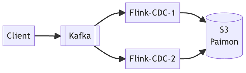
We will start two Flink tasks and keep receiving data from Kafka and writing to the same Paimon table.

The two Flink tasks use different consumer groups, so the amount of data written should be equal.

Therefore, we run the following script in Flink SQL.

1
2
3
4
5
6
7
8
9
10
11
12
13
14
15
16
17
18
19
20
21
22
23
24
25
26
27
28
29
30
31
32
33
34
35
36
37
38

CREATE TABLE orders (  
    order_number BIGINT,  
    price        DECIMAL(32,2),  
    buyer        STRING  
);  
  
CREATE TEMPORARY TABLE kafka_source1 (  
    order_number BIGINT,  
    price        DECIMAL(32,2)  
) WITH (  
    'connector' = 'kafka',  
    'topic' = 'test_topic',  
    'properties.bootstrap.servers' = 'broker:29092',  
    'properties.group.id' = 'session1',  
    'scan.startup.mode' = 'earliest-offset',  
    'format' = 'json'  
);  
INSERT INTO orders  
SELECT  
    *,  
    'session1' AS buyer  
FROM kafka_source1;  
CREATE TEMPORARY TABLE kafka_source2 (  
    order_number BIGINT,  
    price        DECIMAL(32,2)  
) WITH (  
    'connector' = 'kafka',  
    'topic' = 'test_topic',  
    'properties.bootstrap.servers' = 'broker:29092',  
    'properties.group.id' = 'session2',  
    'scan.startup.mode' = 'earliest-offset',  
    'format' = 'json'  
);  
INSERT INTO orders  
SELECT  
    *,  
    'session2' AS buyer  
FROM kafka_source2;

As you can see from the script, I used two kafka sources and wrote to the same orders table, only the buyer field is different. In the end, all we need to do is GROUP BY buyer to know if the two tasks are the same.

Here are some ingest samples.

1
2
3
4

{"order_number": 1, "price": 100}  
{"order_number": 2, "price": 200}  
...  
{"order_number": 100, "price": 10000}

Experiment Result

In the scene where file is used as a metastore, it is easy to see that Flink’s task is constantly restarting.

There are two types of error cases mentioned in the document.

The first one is snapshot conflict.

This will result in a direct data loss, which will be reflected in the following error on Flink.

1
2
3
4
5
6

java.lang.RuntimeException: Exception occurs when committing snapshot #19 (path s3://warehouse/flink/default.db/Orders/snapshot/snapshot-19) by user 2439e7bb-506d-4ff3-a204-ab66610dd75d with identifier 3265 and kind APPEND. Cannot clean up because we can't determine the success.  
	at org.apache.paimon.operation.FileStoreCommitImpl.tryCommitOnce(FileStoreCommitImpl.java:986)  
	at org.apache.paimon.operation.FileStoreCommitImpl.tryCommit(FileStoreCommitImpl.java:715)  
	at org.apache.paimon.operation.FileStoreCommitImpl.commit(FileStoreCommitImpl.java:301)  
  
the rest omitted

Another scenario is files conflict.

This will also cause the Flink task to restart with the following error.

1
2
3
4
5
6

java.lang.RuntimeException: This exception is intentionally thrown after committing the restored checkpoints. By restarting the job we hope that writers can start writing based on these new commits.  
	at org.apache.paimon.flink.sink.RestoreAndFailCommittableStateManager.recover(RestoreAndFailCommittableStateManager.java:84)  
	at org.apache.paimon.flink.sink.RestoreAndFailCommittableStateManager.initializeState(RestoreAndFailCommittableStateManager.java:77)  
	at org.apache.paimon.flink.sink.CommitterOperator.initializeState(CommitterOperator.java:153)  
      
the rest omitted

Either type of conflict will affect the real time ability to write data, or worse, data will be lost in a snapshot conflict.

Solution

Of course, Paimon also provides a solution to this problem, which is to use a metastore that can be locked, such as MySQL.

So in our experiment, we need to change the practice of CREATE CATALOG. The correct CATALOG is shown in README.md, and the key point is to add the following line.

1

'lock.enabled' = 'true'

When we re-run the experiment using MySQL Catalog, we find that both Flink tasks run stably, no longer restarting, and the data in paimon is no longer lost.

Conclusion

In this experiment, we can see that when using two writers to write to the same table, it is very easy to generate conflict even if the amount of data is not large and the write speed is not fast.

If this is the case, it is important to use a metastore that can be locked in any case.

Nevertheless, as of today Trino still does not support jdbc metastore, which will greatly affect the popularity of Paimon, after all, not everyone has Hive in this era.

Originally published on Medium

Deconstructing A/B Test

A practical guide to building custom A/B test frameworks without overhead

When talking about A/B test, many organizations always think of the need for “certain” commercial tools, as if those tools are the only way to implement A/B test.

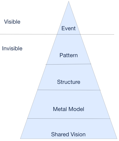
In fact, in the previous article, we talked about systems thinking, and the most important aspect of any system change is a shared vision, followed by a mental model, and the specific tools are at the surface level.

Therefore, the problem with the introduction of the A/B test is the mindset, not the tools.

This article aims to deconstruct the A/B test process and make the introduction of A/B test easier and more natural, without having to rely on a huge enterprise solution.

Breaking Down the A/B Test Workflow

An A/B test experiment consists of the following four core elements.

1. Setting up experiment conditions: Someone needs to design an experiment situation to verify the hypotheses, e.g. we want to test whether the new version of checkout process will increase the conversion rate.
2. Implementing experiment behaviors: The application implements different workflows based on group information.
3. Event logging: Events need to be sent out in different workflows and these events need to contain group information.
4. Post-analysis: Based on the event logs, the analysis is done to determine whether the initial hypothesis is correct or not, and whether the initial experiment conditions are appropriate or not.

Let’s describe an A/B test interaction with a complete time sequence.

1. Front-end receives group information from somewhere.
2. Front-end interacts with back-end with this group information.
3. Either front-end or back-end needs to do something based on the group information.
4. Throughout the process, the events with the group information are sent to the event collector based on the tracking points.
5. The event collector will store all the events for subsequent analysis.

This completes an A/B test interaction, and there will be enough information to analyze it continuously.

Identifying and Addressing Gaps

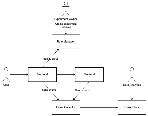
Let’s abstract this whole process to see what components are essential.

I believe front-end and back-end should both exist, so there are three key components.

1. Rule Manager: This is the role to manage the experiments and rules, which is what the first step of the time sequence above refers to somewhere.
2. Event Collector: This is the event collection platform, i.e., the receiver of events sent from front-end or back-end.
3. Event Store: This is where events are stored, either as part of the event collector or as a dataset pulled down through ETL.

For an application developed over a period of time, I feel that event collector and event store should already be in place, after all, even if no A/B test needs, there will be a need for various types of event management.

But for some projects that are just starting out, these two roles may be unfamiliar. However, I have to say that for small projects, the implementation of these two roles can be very simple.

Event collector is actually an api service, and event store is a database. Of course, as the project gets bigger and there are more events, the volume of the event store is likely to become huge, but BigQuery or Redshift can solve many of the difficulties.

So the only thing that really matters is the rule manager.

What is Rule Manager?

A rule is a relatively abstract concept that describes a sequence of logical branches from which we can derive the final result from the inputs.

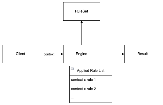
A rule manager, as you can tell from its name, is a role that manages a rule set and processes the inputs and produces the outputs through a rule engine.

Martin Fowler also has an excellent article on rule engine.

Let’s use a concrete example to describe what a rule manager does.

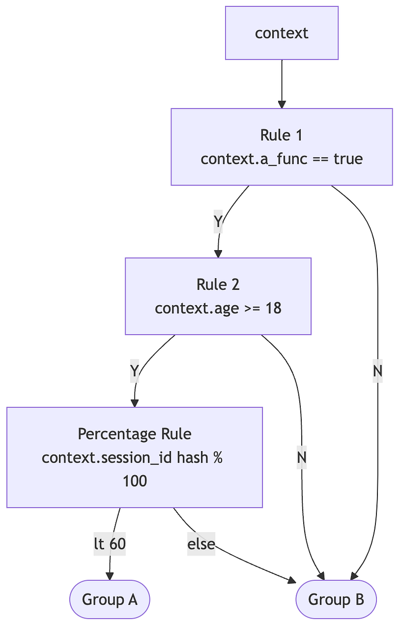
Suppose we want to design an experiment to verify the checkout behavior of adult customers in all stores that have the “A” feature. In this case, we want to set 60% of users who meet the criteria to be A, 40% to be B, and any who do not meet the criteria to be recognized as B by default.

This is an experiment scenario, and we can create a configuration file based on this experiment scenario.

1
2
3
4
5
6

- experiment: test_checkout  
  A:  
    - "a_func = true"  
    - "age >= 18"  
    - "percentage: 60%"  
  default: B

This configuration file creates three rules and relates them to the experiment test_checkout.

Accordingly, we need to create a context on the client side that contains the necessary information for the rule engine to operate on the rules.

Here is a possible context.

1
2
3
4
5

{  
  "session_id": <str>,  
  "a_func": <boolean>,  
  "age": <int>,  
}

Because we have three rules, the context needs to contain three fields, of which session_id is a special one. The other two fields are easy to understand, but what is session_id?

This usually refers to the user’s GUID, which may be user_id or device_id or some other kind of GUID, in order to avoid the possibility that users may be assigned to different groups during a sequence of operations, which would not only pollute the experimentation data, but also make for an inconsistent experience for the users.

In an experiment where we need to assign a specific percentage of users to different groups, there are two ways to accomplish this.

1. Having a record of all the users allows us to accurately assign the ratio.
2. We can get the relative ratio by using a consistent hashing algorithm with a mod.

It is much more difficult to realize the precise ratio than the second approach, so most of the rule engine adopts the relative ratio.

The implementation of a whole rule engine is more difficult depending on the number of supported rules, but if we keep a good code structure, I’m sure it won’t complicate the rule manager.

The following is a simple example, since it uses Chain of Responsibility pattern, it is not difficult to add more rules in the future.

Why Avoid Commercial Tools?

Why do we need to deconstruct the A/B test process? Wouldn’t it be better to just use a ready-made tool?

By deconstruct the A/B test process, we should be able to understand that A/B test is not complicated, and that the function of each component is quite simple. If there are already existing components in the organization that can be reused, even better.

The biggest problem with introducing commercial tools is integration. Those enterprise solutions are end-to-end solutions and require some rewriting of the entire application.

At the initial stage of introducing A/B test, if we are not even familiar with the mentality and methodology of A/B test, we will make drastic changes, which will only result in a greater Resistance to Change.

Moreover, at the beginning, the experiment scenario we design must not be too large and complicated, and we don’t need a very complete solution to realize it.

Take the example in this article as an example, the rules of comparison, equality, and percentage, which are commonly used in A/B tests, can be implemented in just a few lines of code.

Conclusion

I understand that those commercial tools have their strengths and specialties, and I agree that in most cases it’s important not to reinvent the wheel.

However, when we learn from systems thinking that it’s more important to be at the bottom of the iceberg model than at the top, we should look back and see if our current needs are really a wheel.

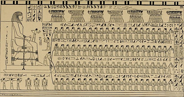
Or can we actually build a pyramid with a sledge?

From my point of view, purchasing an enterprise product involves going through layers and layers of financial reviews, and convincing departments to change existing applications one by one, which involves a huge amount of risk when the results are impossible to estimate.

Therefore, I would choose a relatively simple approach to achieve almost the same result.

Originally published on Medium

Systems Thinking makes software development more efficient

This week I held a few workshops within my organization to explain what Systems Thinking is and some of the common tools used in Systems Thinking, supported by an ongoing classic case study from my organization.

While gathering material for these workshops, two common questions often came up.

1. Will you guide us through the design of an e-commerce system, an instant messaging system, or any system in this workshop?
2. We don’t usually have the opportunity to redesign a system, so do we still need to learn systems thinking?

These questions are closely related. Essentially, they both ask whether Systems Thinking is the same as software architecture design.

The answer is definitely no.

Systems Thinking is a methodology that goes beyond software architecture design and can be applied to any situation and any problem.

So, what exactly is Systems Thinking? How does this relate to our daily routine?

What is System?

Before explaining the importance of Systems Thinking, let’s talk about what a system is.

Simply put, a system is a group of entities that are “interrelated” yet “independent,” working together toward a “common goal.”

The most important part of this sentence is the common goal.

A Chinese proverb describes “a plate of loose sand”, meaning even though everyone in the group is sand and on the same plate, you wouldn’t call it a system because there’s no goal.

Is a baseball team a system? Absolutely. Each member has specific roles, like infielders, outfielders, or pitchers, but they share the common goal of winning.

Now you know a system is not a software architecture.

What Are the Benefits of Learning Systems Thinking?

Let’s go back to the second question at the beginning of this article.

Why do we need to learn Systems Thinking? How will it be applied in daily routine?

While we may rarely get the chance to redesign software architecture — whether through decomposition or changes in data structure — we, as developers, frequently face the challenge of implementing various features and functionalities.

Have you ever thought about how to improve the productivity of your development when you have a large-scale project taking several months to complete?

How do you plan project progress when changes affect multiple files, modules, or even services? How can you batch tasks effectively or minimize the impact radius during a critical failure?

These are all areas of Systems Thinking, and they are issues that every engineer needs to face.

I have written an article in introduction to the decision making process, which is actually a practical application of Systems Thinking.

At the top of the pyramid is the “common goal” of the system.

The following diagram shows the iceberg model of Systems Thinking.

The events we observe in daily routine are just the surface. When things go wrong, how can we address them? Systems Thinking emphasizes that the deeper we delve into the underlying structures and mental models, the greater our influence becomes.

Conclusion

I’m not going to dig into the details of Systems Thinking too much in this article, after all, it’s not something to cover in a few words.

But this article should quickly answer two common questions.

• What is Systems Thinking?
• What are the benefits of learning Systems Thinking?

As software development becomes more complex and chaotic, it feels like venturing into darkness without direction. What we need is a light — a guiding beacon to illuminate our path and help us find clarity. That light is Systems Thinking.

Systems Thinking isn’t a skill limited to architects or managers; it’s a mindset every engineer, product owner, and leader can benefit from. Whether you’re tackling a multi-month project or debugging a critical issue, systems thinking can help you see the bigger picture and guide your decisions with clarity.

Originally published on Medium

A hands-on guide to integrating Apache Paimon, Flink, and Trino for efficient streaming and querying in data lakehouses.

Apache Paimon is a new data lakehouse format that focuses on solving the challenges of streaming scenarios, but also supports batch processing. Overall, Paimon has the potential to replace the existing Iceberg as the new standard for data lakehousing.

Why Iceberg and not the other two (Hudi and Delta Lake)?

Iceberg is the most widely supported by various open-source engines, including pure query engines (e.g., Trino), New SQL databases (e.g., StarRocks, Doris), and streaming frameworks (e.g., Flink, Spark), all of which support Iceberg.

However, Iceberg faces several problems in streaming scenarios, the most serious one is the fragmentation of small files. Queries in data lakehouses rely heavily on file reads, and if a query has to scan many files at once, it will of course perform poorly.

To address this issue, an external orchestrator is required to regularly merge files. Paimon is designed with a built-in merge mechanism, and many other optimizations for mass writes, making it more adaptable to streaming scenarios.

Experiment environment

In order to learn more about Iceberg, I have set up two experimental environments.

• Iceberg + Flink
• Iceberg + Trino

This time I also built a playground for Paimon, which also includes Trino and Flink.

In addition, StarRocks was also put in as a representative of New SQL.

Because neither Trino nor StarRocks support streaming writes at this stage, Paimon’s writes come from Flink.

How to use

NOTE: Since some of the links to the official Paimon files are not working, I’ve put the files into this repo. However, some of the files are huge, so I put them in via LFS, so be sure to install git-lfs.

Trino driver is in paimon-trino-427-0.8-20241112.000605-197-plugin.tar.gz.

1

tar -zxvf paimon-trino-427-0.8-20241112.000605-197-plugin.tar.gz

Then it will run normally with docker compose up -d.

1

docker compose up -d

Flink

Let’s start by connecting to Flink SQL.

1
2

docker compose exec flink-jobmanager ./bin/sql-client.sh  
./bin/sql-client.sh

To write data using Flink we first need to create the correct catalog.

1
2
3
4
5
6
7
8

CREATE CATALOG my_catalog WITH (  
    'type' = 'paimon',  
    'warehouse' = 's3://warehouse/flink',  
    's3.endpoint' = 'http://storage:9000',  
    's3.access-key' = 'admin',  
    's3.secret-key' = 'password',  
    's3.path.style.access' = 'true'  
);

As shown in the above commands, we’re using the MinIO as an S3 to store the Paimon.

The next step in creating the table and writing the data is quite simple, just run the commands according to the official documentat.

1
2
3
4
5
6
7
8
9
10
11
12
13
14
15
16
17
18

USE CATALOG my_catalog;  
  
-- create a word count table  
CREATE TABLE word_count (  
    word STRING PRIMARY KEY NOT ENFORCED,  
    cnt BIGINT  
);  
-- create a word data generator table  
CREATE TEMPORARY TABLE word_table (  
    word STRING  
) WITH (  
    'connector' = 'datagen',  
    'fields.word.length' = '1'  
);  
-- paimon requires checkpoint interval in streaming mode  
SET 'execution.checkpointing.interval' = '10 s';  
-- write streaming data to dynamic table  
INSERT INTO word_count SELECT word, COUNT(*) FROM word_table GROUP BY word;

Then we actually read it and see the result of what we’ve written.

1
2
3
4
5
6
7

-- use tableau result mode  
SET 'sql-client.execution.result-mode' = 'tableau';  
-- switch to batch mode  
RESET 'execution.checkpointing.interval';  
SET 'execution.runtime-mode' = 'batch';  
-- olap query the table  
SELECT * FROM word_count;

Trino

Let’s go to Trino’s cli first.

1

docker compose exec trino trino

Trino’s paimon catalog is already set up, but I didn’t add a new schema but just used the default one.

So we can query the Flink write result directly.

1

SELECT * FROM paimon.default.word_count;

We should see something similar to the Flink query.

StarRocks

This is an extra, just to show how much attention Paimon is getting now that many New SQL databases are starting to support it.

Prepare a mysql client locally to connect to StarRocks.

1

mysql -P 9030 -h 127.0.0.1 -u root --prompt="StarRocks > "

We still need to create a catalog.

1
2
3
4
5
6
7
8
9
10
11

CREATE EXTERNAL CATALOG paimon_catalog_flink  
PROPERTIES  
(  
    "type" = "paimon",  
    "paimon.catalog.type" = "filesystem",  
    "paimon.catalog.warehouse" = "s3://warehouse/flink",  
    "aws.s3.enable_path_style_access" = "true",  
    "aws.s3.endpoint" = "http://storage:9000",  
    "aws.s3.access_key" = "admin",  
    "aws.s3.secret_key" = "password"  
);

The mysql client should not support Trino’s table locator format: <catalog>. <schema>. <table>, so we have to switch to the db before we can query.

1
2

USE paimon_catalog_flink.default;  
SELECT * FROM word_count;

The results here will be similar to the above.

Conclusion

Although Paimon supports many kinds of metastore as follows.

• filesystem
• hive metastore
• jdbc

For the sake of simplicity, I didn’t use extra components, so I only use S3 aka filesystem as metastore. Although the function is fine, according to the official document, using S3 as warehouse needs to be paired with Hive or JDBC metastore to ensure consistency.

But for object storage such as OSS and S3, their ‘RENAME’ does not have atomic semantic. We need to configure Hive or jdbc metastore and enable ‘lock.enabled’ option for the catalog. Otherwise, there may be a chance of losing the snapshot.

My future experiments will focus on understanding the scenarios that require this level of consistency.

Originally published on Medium

Is there an Alternative to Debezium + Kafka?

Evaluating open-source options to improve performance and scalability in CDC pipelines

I asked this question on Reddit a while back and received lots of valuable answers.

Therefore, I’ve looked into each answer and documented the results in this article.

TL;DR

No, Debezium dominates the market at the moment, despite some drawbacks.

Background Explanation

Why would we want to find an alternative to Debezium? The main reason is we encountered a challenging scenario.

This is a typical scenario for Debezium, where any modifications to the data source are captured and fed into Kafka for downstream processing.

The advantage of this architecture is simple and efficient, ensuring all downstream processes are as real-time as possible.

If the source has a large number of updates, Debezium can scale horizontally until a large number of updates are concentrated in a single table. This is where Debezium hits its limits.

Even though Debezium can scale horizontally, it means the updates originally handled by one process can be distributed to multiple processes. If each table already has a dedicated process, horizontal scaling is no longer feasible.

We are in such a situation, in our environment, even if the machine specification is stretched, the CDC throughput of a single table is capped at 25 MB/s.

This is certainly not a regular case, after all, 25 MB/s change for a single table is quite significant. However, if we encounter a data source that is doing large-scale data migration, this limit can be easily breached.

In order to ensure the real-time performance of our data pipeline downstream, we can only ask the upstream to be merciful when encountering this level of data migration, and try to do a good job of rate limiting.

However, this limitation will greatly reduce the productivity of the upstream developers. On the one hand, they have to add auditing process to their regular maintenance, and on the other hand, they need to develop an additional rate limit for each maintenance.

So let’s find a solution.

Solution Overview

The following solutions were gathered from that Reddit article.

1. Estuary Flow
2. Striim
3. Fivetran HVR
4. Proprietary CDC
5. Conduit

The first three solutions are enterprise services without open source, so they’re not going to work for us. After all, we’re trying to solve a partial use case, not a complete do-over.

Although Estuary Flow says they have a local deployment approach, I couldn’t find any information about it.

The fourth solution was to develop a new tool ourselves, which I believe would be a fundamental solution to the problem. After all, Debezium is developed in JAVA, and we should be able to achieve better performance with Golang, Rust, or even C/C++. However, the development cost was too high for us, and it was difficult to start from scratch.

The first four options didn’t meet our needs, but the fifth option caught my attention as a promising solution.

Conduit is an open source data migration platform developed in Golang, and provides a variety of connectors to integrate many data stores. In addition, we can also develop our own converter to do data format preprocessing.

Therefore, I started to test the performance of Conduit.

Expirement Environment

To keep things simple, I used Kafka Connect in place of Debezium. The two are essentially the same but with different dispatchers, and behind the scenes they all use the same library.

Locust is responsible for generating MongoDB changes, then Conduit and Kafka Connect will write to different Kafka topics.

We can observe the writing speed of Kafka topics to determine who has better performance.

The whole experiment environment is as follows.

I use two of my own packaged images, Conduit and Kafka Connect, which have MongoDB connectors.

• Conduit + Mongo connector
• Kafka Connect + Mongo connector

It’s easy to generate a large amount of change by stuffing MongoDB with a bunch of fat documents and then just changing the value of a field in all the documents.

The locust script used is as follows.

1
2
3
4
5
6
7
8
9
10
11
12
13
14
15
16
17
18
19
20
21
22
23
24
25
26
27
28
29
30
31
32
33
34
35
36
37
38
39
40
41
42

import time  
  
from locust import User, task, between  
import pymongo  
  
class MongoDBUser(User):  
    wait_time = between(1, 5)  
  
    def __init__(self, environment):  
        super().__init__(environment)  
        self.env = environment  
  
    def on_start(self):  
        self.client = pymongo.MongoClient(self.host)  
        self.db = self.client["test"]  
        self.collection = self.db["test_new"]  
      
    @task  
    def incr_seq(self):  
        response = None  
        exception = None  
        start_perf_counter = time.perf_counter()  
        response_length = 0  
  
        try:  
            response = self.collection.update_many(  
                {},  
                {"$inc": {"seq": 1}}  
            )  
            response_length = response.matched_count  
        except Exception as e:  
            exception = e  
  
        self.env.events.request.fire(  
            request_type="mongo",  
            name="incr seq",  
            response_time=(time.perf_counter() - start_perf_counter) * 1000,  
            response_length=response_length,  
            response=response,  
            context=None,  
            exception=exception,  
        )

Load Test Result

For this test, I used a local machine without fully stressing its CPU or memory, leaving some resources available to avoid errors from performance bottlenecks.

In other words, this test shows the regular ability of a single process to handle a single table load.

As the results show, Kafka Connect’s throughput significantly outperforms Conduit’s when system resources are sufficient.

I was a bit confused about this result, so I repeated the test a few times, but I got similar numbers.

Wrap Up

Back to the question in the title.

Is there an alternative to Debezium + Kafka?

Not at the moment — at least, not among open-source tools.

I’ve asked on Reddit, but maybe Medium will have a different answer, so feel free to offer your solutions.

Originally published on Medium