The difference between the perspective of a backend engineer and a data engineer
Although I have been working with data in the past, this year, I have been working closely with data engineers and finally fully realized the concept of data-centric.
We all know that applications are made up of data, so as a backend engineer or architect, we must be involved in all kinds of data storage and data structures. How to get the most efficiency out of all kinds of data storage is the goal of every backend engineer, and our focus is on maximizing the throughput of data storage with the most efficient data structures.
There are many technical details involved, including but not limited to the following.
But for data engineers, the focus is completely different.
How to find the answer to a question quickly with a lot of data at hand?
Quick here has a very different meaning to what a backend engineer cares about. Data engineers care about quickness in terms of productivity, so they can use all kinds of complex SQL queries, let’s say over 100 lines, to find the answer, even though the SQL query takes a long time.
This is the opposite of what the backend engineers care about, which is the speed of response. From the backend engineer’s point of view, such a complex and time-consuming query is unimaginable.
Data engineers have different data requirements in order to achieve their goals.
ETL and ELT: make data more structured.
Data Lakehouse: continuous data cleanup and compilation.
Governance: manage data catalogs and lineages.
How to organize the data from many sources into a structure that is suitable for use, and put it in an easy-to-access place and reduce the complexity of maintenance is the focus of data engineers.
Therefore, let me summarize this year’s experience in one sentence.
Only those who focus on data and care about data are data engineers.
This is the meaning behind data-centric, and I have spent a lot of time this year learning and changing my mindset in order to understand this.
Data-centric Monitoring
In fact, the concerns of backend engineers and data engineers are also reflected in the metrics of the monitoring system.
The application quality metrics usually include the following key points.
response latency
throughput
error rate
However, for data applications, the quality metrics will be as follows.
Freshness: time lag between source and landing.
Completeness: whether data is lost at each stage of transformation.
Correctness: similar to the above, whether each stage of transformation is correct.
Although, both are applications, they are very different for telemetry. Of course, the underlying infrastructure is also different.
Data Team Organizations
Let’s break down the composition of a data team.
From my point of view, a complete data team would have at least two roles with completely different skill sets and totally different responsibilities: data engineer and data analyst.
In my opinion, there is a simple dichotomy between how to differentiate these two roles.
Data Analyst: the person who uses data to answer questions.
Data Engineer: the person who generates the “data” above.
Of course, there are two other roles that can be created depending on how the questions are answered.
Data Scientist: the person who answers the question through himself.
Machine learning engineer: answers questions through AI.
But for a healthy data team, I believe there needs to be at least a distinction between the roles of data engineer and data analyst. Just as the focus of a backend engineer is different from that of a data engineer, the focus of a data engineer is different from that of a data analyst.
Conclusion
Throughout 2022, I learned a lot of new experiences and was able to find my blind spots in my domain knowledge in a new role.
As an architect, I believe I still have a lot to learn, so please continue to share and discuss with me in the new year.
Demonstrating some common practices of SQL Window Function
When doing ETL, we always write data into the database one batch at a time, which contains the snapshot of each batch. these snapshots are basically historical data and may contain a lot of duplicates, so how do we find the data we need in these batches?
This article will use a simple scenario to describe some of our common processing methods, mainly window function.
User Scenario
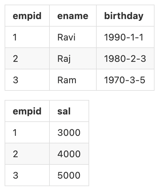
Suppose a company uses a BPM system to manage employee changes and salary changes, then a simple BPM system will usually have two tables with the details of the employee and the salary of each person as follows.
When working with relational databases, we usually normalize the data, i.e., we plan the tables in terms of requirement dimensions and keep only the necessary fields, which are related to each other by foreign keys.
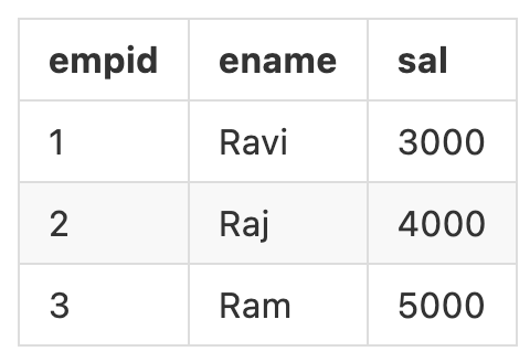
But in the data analysis context, we often need a fact table, which means everything is aggregated together. An example of a fact table for salary analysis might look like the following.
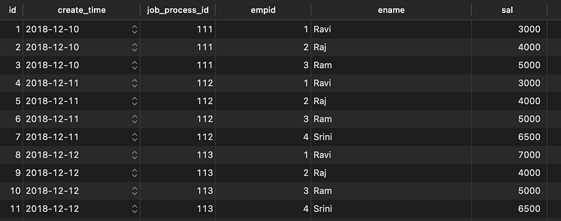
The common practice in aggregation is batch processing ETL, where each time the required columns are fetched from the employee details table and salary table and saved for later analysis such as salary increase trend. The fact table after the ETL aggregation is as follows.
This is an ETL for batch processing in days, and the two tables will be aggregated every day, so there will be job_process_id for batch processing and create_time for data creation.
As we can see from the above figure, the fact table generated by ETL will contain a lot of duplicate data, if we need to know the current state and to exclude duplicates, how to do? This is where the window function comes into play.
1 2 3 4 5 6 7 8 9 10 11
SELECT t.* FROM ( SELECT cdc_test.*, (ROW_NUMBER() OVER (PARTITIONBY empid, ename ORDERBY create_time DESC)) AS seqnum FROM cdc_test) t WHERE t.seqnum =1;
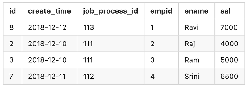
By using PARTITION BY to lock the fixed columns (empid, ename), and sorting the time in reverse order, we can know the first one will be the latest state.
The result is as follows.
Get changes per salary
With the latest state, we usually still want to know about every salary change. We can still achieve our goal through the window function.
1 2 3 4 5 6 7 8 9 10 11 12
SELECT t.* FROM ( SELECT cdc_test.*, (ROW_NUMBER() OVER (PARTITIONBY empid, ename, sal ORDERBY create_time)) AS seqnum FROM cdc_test) t WHERE t.seqnum =1
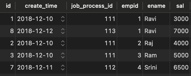
This time, we PARTITION BY to lock the target is (empid, ename, sal), because we want to treat the same three columns as the same group, then once the sal changes will create a new group.
From the results, we can see that Ravi got one raise, from 3000 to 7000.
Get changes per salary and include the result before salary increase
In the above two examples, we only use ROW_NUMBER(), but in fact there are many other functions available in the window function.
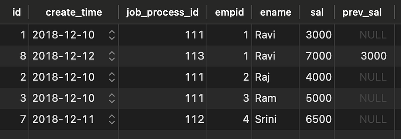
This time, we not only want to get the salary change, but also want the query result to include the column before the salary increase, so we can use LAG().
1 2 3 4 5 6 7 8 9 10 11 12
SELECT t.* FROM ( SELECT cdc_test.*, (LAG(sal) OVER (PARTITIONBY empid, ename ORDERBY create_time)) AS prev_sal FROM cdc_test) t WHERE prev_sal ISNULL OR prev_sal <> sal;
Similar to the above, except that another window function is used and the WHERE clause is changed.
Three Pagination Approaches with SQL and ElasticSearch Demonstration
Pagination is a common technique for web page presentation. When there is a lot of returned data, either to reduce the load on the backend or to improve the user experience, it is usually a good idea to limit the amount of presentation and keep the option to continue browsing.
Here’s a quick look at the most common appearance.
< [1] | 2 | 3 | 4 | ... >
The user can know the current page number, choose the previous or next page, or even jump directly to the specified page. There are three types of pagination approaches as follows.
Offset Pagination
Keyset Pagination
Cursor-based Pagination
But this article is to introduce ElasticSearch pagination, so I will briefly describe these three.
Offset Pagination
This is the most common pagination pattern, and let’s represent it in SQL.
1 2 3
SELECT* FROM table_name LIMIT 10OFFSET20;
Suppose there are 10 records on one page, then we can get the result of the third page by this command. Use LIMIT to limit the number of records per page and use OFFSET to jump to the specified page.
There are many advantages of such a pagination.
It is very easy to implement, as well as very intuitive.
It is possible to jump to a random page.
But the disadvantages are also obvious.
Performance is a problem.
Why is there a performance problem?
In the above example, it looks like we only need to take 10 records from the database, but in fact, the database will take 30 records and discard the first 20 records. When OFFSET is very large then the database will still take all the records and create a lot of overhead.
Keyset Pagination
In order to solve the performance problem, we have the keyset pagination approach.
We still use SQL as an example, following the above scenario, we limit the number of records per page to 10 and take the third page.
1 2 3 4 5
SELECT* FROM table_name WHERE id >20 ORDERBY id LIMIT 10;
Using LIMIT to limit the number of records per page is the same as above, except that we first sort by ORDER BY and then set the starting position by WHERE instead of OFFSET. In this way, we can get the third page without taking 30 records.
There are several implementation details that must be paid attention.
Must be able to sort quickly, in the case of relational databases, the columns to be sorted must have indexes.
Where do the WHERE clause come from? It can be from the frontend with the last position of pages, or it can be the backend through some storage mechanism.
Of course, there are advantages and disadvantages to such a pagination. The advantages are as follows.
It works well when implemented correctly, e.g., on index columns.
It can run on very large data sets.
But these advantages come at a price.
difficult to implement
no way to jump to random pages
I believe the first drawback is easy to understand, after all, it is not a very intuitive approach, the WHERE clause is determined by engineering methods.
The second drawback is to jump to a specific page, there must be a correct WHERE clause, but this WHERE clause depends on the last page jump result, whether it is frontend or backend processing. Therefore, users cannot jump pages as they wish.
Cursor-based Pagination
This is an advanced version of keyset pagination, which is actually a special case of cursor-based pagination.
A cursor is an object defined by the engineering side to mark where the pagination starts. There are several common types of cursors.
Encoded cursor, such as base64. Suppose the cursor is eyJpZCI6IDIwfQ==, then we will find out it is a JSON format string and the specified id is 20.
Token cursor, the backend generates a token for each search result and stores the token, the frontend can use the token to specify the jump page, the backend can know where to start from based on the token.
No matter which cursor is used, the backend still uses the keyset pagination mechanism for pagination.
The advantages and disadvantages of cursor-based pagination are fully inherited from keyset pagination, but cursor has the extra advantage that cursor can store more information, such as session timeout, user privilege, etc.
How about ElasticSearch
The examples above use SQL as an example, but in fact ElasticSearch supports these methods as well.
Similar to the principle of SQL, from is used to specify where to start, and size is used to limit the number of records per page. Then, of course, there are also scalability limitations, and moreover, ElasticSearch directly limits the maximum amount of from and size in order to avoid poorly performing queries from affecting the health of the cluster.
max_result_window: The maximum amount of data that can be searched at once, the default is 10000. If from + size > 10000, it will directly return an error.
How to solve it? Use the keyword search_after for keyset pagination.
This is a typical implementation of keyset pagination on ElasticSearch.
So does ElasticSearch have support for cursor-based pagination? Yes, and unlike SQL, you have to implement your own cursor in the application. ElasticSearch already has its own cursor mechanism, called the Scroll API.
The principle is to create a snapshot of the current query and jump to the next page by calling scroll every time. A practical example would look like the following one.
This will get a response with _scroll_id, and then we can jump to the next page just by using this _scroll_id.
1 2 3 4 5
POST /_search/scroll { "scroll": "1m", "scroll_id": "OXOXQQ==" }
Since it is a cursor-based pagination, we cannot specify which page we want to jump to, we can only keep going to the next page until there is no result.
Because Scroll API is a snapshot of the current query result, so we must carefully choose the TTL or delete the snapshot after finishing, otherwise it will occupy the hard drive space.
In the new version of ElasticSearch, it is no longer recommended to use Scroll API for deep pagination, instead, another new mechanism (released after 7.10), PIT (Point In Time).
PIT works similarly to Scroll API, but is more flexible and better optimized for performance.
Scroll API takes a snapshot of a single query and can only jump pages on that snapshot, but PIT takes a snapshot of the current data set and can do anything after getting the snapshot, not just jump pages.
However, this is not related to the pagination, so I will not dive into PIT in this article.
Conclusion
In general, there are two major types of pagination, offset pagination and keyset pagination, and only keyset pagination can run on big data, but if you want to jump pages randomly, only offset pagination can, which is a trade-off.
In fact, in a big data scenario, if the feature requirements strictly define the maximum number of pages, then even using offset pagination will not affect performance.
Therefore, it is not just a technical decision to choose the implementation method, but more often a trade-off in terms of feature requirements. Nevertheless, engineers should know if there is a requirement for random page jumping on big data without page limit, it is time to say no, please clearly reject.
A statistical solution to know if its time to refactor your code
API slowdown has a great impact on the user experience or even loss of trust, so we always want to know the latency as early as possible.
Therefore, it is common to integrate performance tests and measurement benchmarks into automation testing.
But the concept of slow is very difficult to evaluate.
Did it happen by accident? Or is it an ongoing status?
Is it caused by the experimental environment? Or is it a side effect of the code?
Is it the result of increased features? Or is it a defect?
It is difficult to have a clear answer to these questions.
Assuming we have a way to detect “slow”, then we will send an alarm or a report. But if it’s just a “coincidence” or a false alarm caused by experimental environments, eventually people will try to ignore these signals.
In addition, it is to be expected that APIs will slow down as features are added. When we have more parameters, more business logic, and more if-else, it’s no wonder that the response time slows down.
Furthermore, if we use threshold to avoid the above problem, then when we really recognize API slowdown, we won’t know what the root cause of the slowdown is.
All these factors make the task of detecting API slowdowns extremely hard.
It’s time for statistics to come into play
To address the mentioned issues, let’s summarize the requirements.
to be able to know specifically when the problem occurs
to be able to allow accidental outliers
to be able to avoid the normal phenomenon of slow rise
to be able to issue alarms
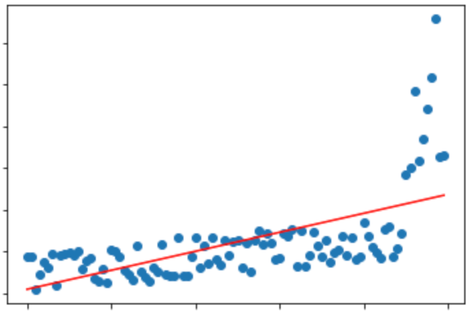
First, let’s look at a diagram.
The horizontal axis indicates each test, which can be considered as time or release version, or even if integrated into CI/CD pipeline, that is each commit.
The vertical axis is the latency of the target tests.
The red line is the main character of this article, Linear Regression.
From the diagram, we can know before a certain time, basically the latency is slowly increasing, but after a certain time, the whole latency is rapidly increasing. And that time point is the problem we want to know.
Perhaps you will say, it is easy to find out by the naked eye by looking at the numbers each time? After all, it is quite intuitive.
The key is the scale of the latency. If the average of the data points from the group below is 0.1 seconds, and the group behind is 0.2 seconds, will you still feel very intuitive?
Therefore, we need a brain-friendly standard, i.e., linear regression.
Through linear regression, we can know the overall trend of the data set is up. However, this is not enough, because just knowing that the trend is up does not mean we can judge whether it is normal or abnormal.
The group of dense data points in the front is also up, so how can we determine that the trend is abnormal and the front is normal?
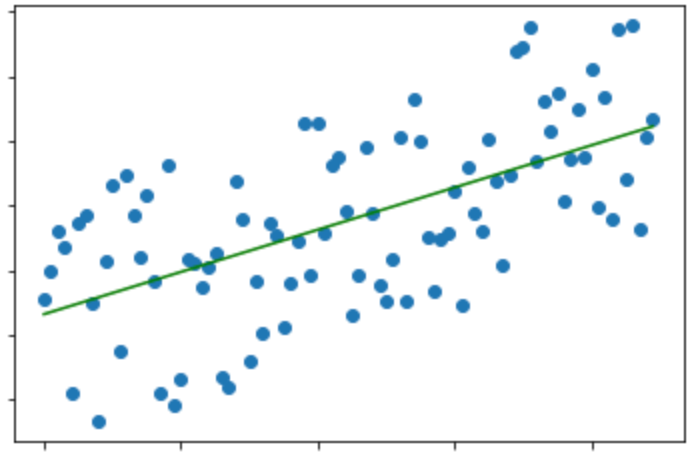
Let’s look at another diagram.
Question: Is the latency of this diagram normal or abnormal?
It looks very similar to the previous diagram, there is a clear upward trend, so it should be abnormal, right? Really?
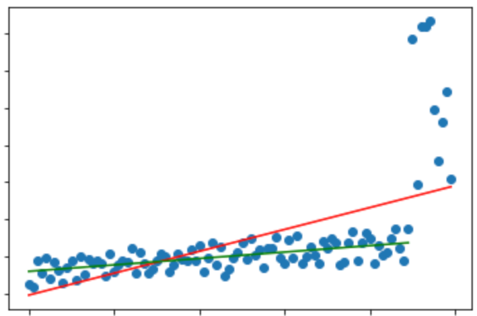
Let’s add some reference points and zoom out a bit.
Have you found? The diagram above is actually a normal part of the original diagram, just a slow rise.
By simply doing linear regression analysis on a single data set, we may get wrong conclusions because we have no benchmark for comparison and cannot tell whether it is a natural phenomenon caused by increased features or a problem caused by defects.
Solution
Back to our question, how can we detect the problem as early as possible without false positives?
First, we need to choose a reference point, e.g., one day ago. Then, we perform a linear regression on the entire data to get a red line. Of course, we also need to perform a linear regression on the data before the reference point, which will lead to the green line.
The slope of the red line and the green line is used to calculate the angle as the judgment basis. In other words, when the angle between the red line and the green line is larger, then it is more likely to be abnormal.
Therefore, the threshold for setting an alarm is neither the latency itself nor the slope, but the angle of the two lines.
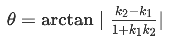
Given the slopes of the two lines are k1 and k2, then the formula for the angle θ is as follows.
In Python, it would be:
1 2 3 4 5
import math thera = math.degrees(math.atan2(abs(k2 - k1), abs(1 + k1 * k2))) # atan2 does not need to handle denominator zero error cases # If we use atan # we need to solve the case where k1 * k2 is equal to -1 first
We can do several experiments with simulated values to get our ideal alarm threshold.
Finally, in addition to the angle threshold, we also need another alarm indicator, which is the upper bound of the allowed latency.
Why do we need to set an upper bound?
Because if our latency keeps increasing in a green line trend, one day it will reach an unacceptable value, but if we just set the angle threshold, we will never know how bad the situation is until we have a disaster on the production.
Finally, the following is an example of how to compute linear regression in Python.
1 2 3 4 5 6 7 8 9 10 11 12 13 14
import numpy as np from sklearn.linear_model import LinearRegression # raw_x and raw_y are the results of each test # raw_x can be a time, version or commit normalization # raw_y are latencies x = np.array(raw_x)[:, np.newaxis] y = np.array(raw_y)[:, np.newaxis] bfl = LinearRegression() bfl.fit(x,y) y_pred = bfl.predict(x) slope = bfl.coef_[0, 0]
Conclusion
So, how do we know if the API is slowing down? We need two alerts.
the angle between the current data line and the data line of the reference point after linear regression.
the maximum upper bound of the latency.
When we have these two alarms, we can know exactly when the code is causing problems and if it is time to refactor the system.
In fact, this is a statistical approach to achieve the goal, but there are still some drawbacks to this. For example, how to set the threshold value of the slope angle? How to choose the reference point? What is the statistical range to be chosen? All these questions require experiments to find the answers.
Therefore, the most effective way is to introduce machine learning into the system of latency analysis, and judge whether the current result is normal or abnormal through the prediction model, rather than through human settings. It’s more difficult for humans to make judgments than machines.
However, to build a machine learning model requires corresponding domain knowledge and skills, which may not be suitable for small organizations, so linear regression is a reliable and low-cost solution.
The Infrastructure Stack for Real-Time Data Analysis
A look at the popular options available
Previously, we introduced the evolution of data infrastructure, where we evolved the original data monolith step by step into an architecture that can support both real time analysis and various data governance.
However, in that article, we didn’t cover what technical selections were available but only a high-level view of the architecture evolution process.
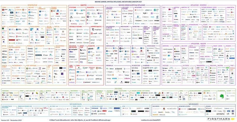
In this article, we will focus on the stack of real-time analysis and list some hot or gradually popular options.
Real-Time Infra
Before starting, let’s briefly introduce the whole architecture of real-time analysis.
As we mentioned before, the core of the entire real-time infrastructure is streaming.
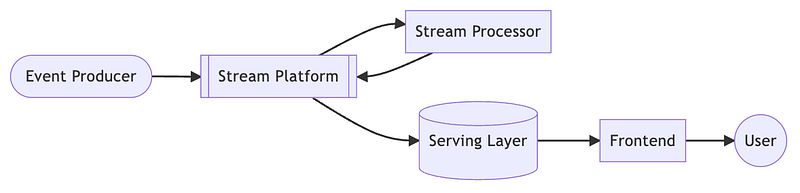
In order to quickly process all events from event producers, streaming plays an important role, and within streaming, there are stream platforms and stream processors. Stream platform is the broker of streaming, which is used to store and distribute streams to processors. And the processor will send the stream back to the platform after processing the stream.
Why don’t processors deliver the streams directly backwards?
Because the stream may go through more than one processor. To complete a full use case, the stream may go through many processors, each of them focusing on what they are intended to do. This is the same concept as a data pipeline.
When the streaming is processed, it is persisted and is available for users as needed. Therefore, the serving layer must be a data store with high throughput and provide a variety of complex queries. For this requirement, traditional RDBMS cannot meet the throughput requirements, so the serving layer is usually not a relational database.
The final front is for presenting the data to the end-user, which can be tables, diagrams, or even a complete report.
Event Producer
We already know that event producer are responsible for generating various “events”, but what kinds of events exactly are there?
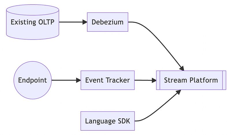
There are three types.
Existing OLTP database
Event tracker
Language SDK
Existing OLTP database
Any system will have a database, whether it is a relational database or a NoSQL database, and as long as the application has storage requirements, it will use the database that suits its needs.
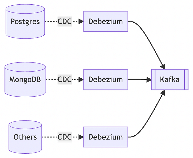
To capture data changes from these databases and deliver them to the streaming platform, we often use Debezium.
Event tracker
When a user operates a system, whether it is a web frontend or a mobile application, we always want to capture those events for subsequent analysis of user behavior.
We want the trackers to be able to digest the rapidly generated events for us, but we also want them to have some customization, such as enriching the events. Therefore, plug-ins and customization will be a priority when selecting a tracker.
SNOWPLOW provides an open source version, while segment does not.
Language SDK
The last is the events generated by various application backends, which are delivered through the SDK provided by the stream platform. The technical selection here will depend on the stream platform and the programming language in use.
Stream Platform
The concept of stream platform is very simple, it is a broker with high throughput.
The most common option is Kafka, but there are also various open-source software and managed services. By the way, the following order does not represent the recommendation order.
A stream processor, as the name implies, is a role that handles streams. It must have scalability, availability, and fault tolerance, and the ability to support various data sources and sinks is also an important consideration.
The Apache Flink, which is often mentioned, is one of these options, and there are many others.
The function of the serving layer is to persist the results of the stream processing and make them easily available to users. Therefore, it must have two important conditions, first, a large throughput, and second, the ability to support more complex query operations.
In general, there are two different approaches, one is to choose a common NoSQL database, such as MongoDB, ElasticSearch or Apache Cassandra. All of these NoSQL databases have good scalability and can support complex queries. In addition, these databases are very mature, so the learning curve is low for both use and operation.
In addition, there are also some NoSQL databases rising up for low latency and big data, e.g., SCYLLA.
On the other hand, there are many newcomers to the SQL family. These new SQL-compatible databases have a completely different implementation logic than traditional relational databases, and thus have a high throughput and can even interact directly with stream platforms.
Moreover, these databases have the scalability that traditional RDBMSs do not have, and can still have low query latency in big data scenarios.
Furthermore, low-code frameworks are becoming popular in recent years. Low code means developers only need to write a small amount of code to use plenty of pre-defined functions, which can significantly shorten the development time and speed up the release.
In order to make the data more real-time, the purpose is to make the value of the data as early as possible, so agile development in the production environment is also a reasonable consideration. Here are two popular low-code frameworks.
Although this article lists a lot of targets for technical selection, there are definitely others that I haven’t listed, which may be either outdated, less-used options such as Apache Storm or out of my radar from the beginning, like Java ecosystem.
Besides, I did not put links to the three major public cloud platforms that are already relatively mature (AWS, GCP, Azure), because those can be found in many resources on the Internet at any time.
Even though these technical stacks are listed by category, some fields actually overlap. For example, although Materialize is classified as a stream processor, it makes sense to treat as a serving layer because it is essentially a streaming database, and the same is true for ksqlDB.
Each project has its own strengths and applications. When making a choice, it is important to consider the existing practices and stacks within the organization, as well as the objectives that you want to accomplish, so that you can find the right answer among the many options.
If there is a project I didn’t list and you feel it is worth mentioning, please feel free to leave me a comment and I will find time to survey it.
Insights from Worldwide Software Architecture Summit vol.2
Six months ago, I attended Worldwide Software Architecture Summit (WSAS’22), where many sessions were discussing complexity, especially the complexity of microservices. At that time, I wrote two insights as follows.
The main point is building a microservice architecture is not always the best solution, the complexity of microservice architecture is very high and there are many trade-offs, how to find a relatively good option among many choices is a challenge.
Recently, WSAS’22 was held for the second half of the year, and I also attended.
Among those sessions, Conway’s Law was mentioned several times.
In order to maintain the microservice architecture, the organization structure also needs to be adjusted to properly maintain many services. In the reorganization, how to let engineers do their work more efficiently also became an important issue.
During the three-day session, I came to one conclusion.
The productivity of engineers can only be increased by focusing on the happiness of engineers.
How to do that? Well, it’s not that hard.
Optimize the onboarding process. Let new engineers get into work mode faster.
Be able to local development. Although the software architecture is moving towards microservices, engineers need to be able to build a development environment with the equipment at hand.
Establish software testing, whether it is unit testing, integration testing or even continuous integration, having a good testing framework to find defects as early as possible will make people more motivated.
Reduce the cognitive load. This covers a wide range of topics, including complete documentation to guide engineers, service templates to reduce the initial process of developing a new service, and a good continuous deployment process to reduce the background knowledge on operations.
Have the permission to do whatever needs to be done, otherwise it will be stuck in various approval processes.
These five items are more from the engineer’s point of view and I believe they are easy to understand.
If you can focus on what needs to be done and have a good way to get it done, then the engineer should be happy.
But there is another item I feel is the most important.
Improving the code quality.
I believe we can all agree poor code can have a serious impact on productivity, but how much? Is there any way to measure it?
One session is a static scanning company, they published a paper, which mentioned that
15 times more bugs in poor code than good code.
the development speed of poor code is 2 times slower than good code.
the feature delivery time of poor code is 9 times longer than that of good code.
From these supporting evidence, it is also indirectly proven that if an engineer has to suffer from poor code, he will not be happy.
From my point of view, microservice governance is much more important than microservice architecture. As an architect, I put more emphasis on how to practice than the perfect architecture. An architecture that makes engineers happy is a good architecture, whether it’s a monolith or a microservice.
However, we also mentioned that each of the three approaches has its own applicable scenario and its corresponding potential risks. So is there a way to extract the advantages of each and construct a more complete solution?
This article will provide an example and explain my ideas.
Solution Concept
Extending the cache time effectively improves the availability of the cache. When the cache is not valid and is requested at the same time, only one request can get through the cache and into the backend system. The rest of the requests will get the original result as the cache time is extended.
However, when concurrent requests occur at the same time ( which is generally uncommon), there is still the possibility of multiple requests entering the backend system, hence the exclusive lock approach.
Nevertheless, the cost of using exclusive locks all the time is too high, and we should try to minimize the use of exclusive locks if possible. Then, use the exclusive lock only when the cache does not exist and there is a need to access the backend system, else just use the extend cache time.
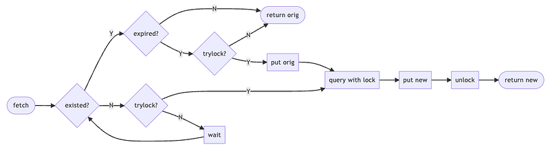
The whole process is as follows.
First of all, determine whether the cache exists, if the cache exists we still have to determine whether the cache is expired. If everything is fine, we can just take the original value of the cache, but if the cache is expired, we must enter the process of updating the cache.
In order to avoid the impact of high concurrent requests, all update cache processes should try to acquire a lock.
On the other hand, if the cache does not exist from the beginning, then the process of updating the cache will be the same. Only the process is different as mentioned above, because there is no original value, so those who did not acquire the lock must wait for the lock before they can get the result.
Solution Overview
Before we get into the details of the implementation, let’s look at the actual practice.
This is an example in Python where we use a decorator to encapsulate an actual database operation.
This decorator requires several parameters.
ttl, this is easy to understand, it is the expiry time of this cache.
lock_period, because we need to acquire the lock, so this parameter determines how long we have to lock.
race_period, this parameter is used to determine how long we want to extend the cache.
In the above example, foo has a cache expiry time of 5 minutes and retains a 1 minute buffer. The lock time is 30 seconds, which is related to the expected time of the database operation.
Solution Details
Next, let’s break down the actual details of the flowchart.
At the beginning of the flowchart, we need to try to get a cache first and use the results to see if we need to extend the cache time.
The top and bottom paths of the flowchart are encapsulated by each class. Let’s look at the implementation of ExistedCacheHandler first.
1 2 3 4 5 6 7 8 9
classExistedCacheHandler(BaseCacheHandler): defhandle(self, func, *args, **kw): if self.now > self.expired_at and Store.try_lock(self.key, self.lock_period): result = func(*args, **kw) Store.set(self.key, result, self.ttl + self.race_period) Store.unlock(self.key) return result return self.orig_val
If a cache has expired and successfully acquires a lock, it is responsible for updating the cache.
In the previous article, we introduced the Rails approach, where Rails writes the original value back to the cache again and extends the valid time slightly. But here, we directly let the cache time be (ttl + race_period), so we don’t need to extend the cache time manually.
On the contrary, if the cache has not expired or has not been locked, then the original result in the cache is used.
On the other hand, the logic of cache not exist is more complicated.
1 2 3 4 5 6 7 8 9 10 11 12 13 14 15 16
classNonExistedCacheHandler(BaseCacheHandler): defhandle(self, func, *args, **kw): while self.expired_at isNone: if Store.try_lock(self.key, self.lock_period): result = func(*args, **kw) Store.set(self.key, result, self.ttl + self.race_period) Store.unlock(self.key) return result else: whilenot Store.try_lock(self.key, self.lock_period): time.sleep(0.01) self.orig_val, self.expired_at = Store.get(self.key) Store.unlock(self.key) else: return self.orig_val
When a cache is found to be non-existed, we still have to acquire the lock in order to update the cache. But if the lock is not acquired successfully, we must wait, either for the lock or for the cache to be updated.
Why should we wait for either of these two conditions?
The reason is the person who acquired the lock may not have released the lock for “some reason”. Our ultimate goal is to get the cache result, so even if we don’t get the lock, we still get the result. Of course, if the lock is successfully acquired, the responsibility of updating the cache will be taken up.
The BaseCacheHandler defines the constructors and a helper function.
Store is the core of the whole implementation, and I use Redis as a demonstration.
get(): In addition to getting the cache value, we also need to get the expiry time of the cache.
set(): Write the value and also set the expiry time.
try_lock(): Use Redis’ atomic update to lock with NX.
unlock(): simply removes the key.
By assembling all these pieces, the cache decorator is complete, not only with the ability to extend the cache time but also with exclusive lock support.
Conclusion
This is a workable example, and we have arranged it in a more intuitive way to make it easier to understand. However, there are some things that could be refined.
For example, many places currently use a single command to operate Redis directly, and it would be better to write it in Redis pipeline. Moreover, it would be a good idea to write some simple logic as a script in Lua.
I have to say such an implementation is actually very complex, but does a read-aside cache really need to do that?
It depends on the load of the application and what we expect from the application.
If the backend system is strong and can handle a sudden spike, then a regular extended cache time can work. But if the backend is weak, it is necessary to consider a more solid approach.
Enhancing the caching mechanism is one option, but enhancing the backend system is also an option. There are several common ways to enhance the availability of the backend system.
circuit breaker pattern
service degradation
multi-layer caching
This article provides an option to enhance the cache, without the need to deploy new components and just modify the logic, in my opinion, it is still worth it.
We have discussed cache consistency before, and at that time we mentioned it is possible to achieve good consistency if we implement read-aside cache correctly. To further improve consistency, a more complex solution must be used, e.g., write through cache or write behind cache.
Today, we are going to discuss another common scenario of caching, Dogpile Effect.
Dogpile Effect means when the system is under heavy volume of traffic, whenever a cache invalidates, either by cleanup or timeout, it will have a huge impact.
For example, if a cache entry is accessed by 100 requests at the same time, once the entry expires, 100 requests will hit the backend system directly, which is a serious challenge for the backend system.
Therefore, let’s see what approaches are available to deal with Dogpile Effect. There are three common approaches as follows.
Warm Up Cache
Extend Cache Time
Exclusive Lock
Each of these three options has its own pros and cons, and in fact, they are already widely used.
Question, do you know which one is therace_condition_ttlof the cache store in Ruby on Rails*?*
Warm Up Cache
Before we talk about this approach, let’s review the read path of the read-aside cache.
First, all read requests are read from the cache.
If the cache fails to read.
Then read from the database, and write back to the cache.
The problem occurs when the cache is missed.
When there are lots of read requests under a high volume system, it will result in lots of database accesses. If we can keep the cache active anyway, can’t we solve Dogpile Effect?
Thus, the approach is to replace the cache TTL with a background thread that updates all caches periodically, e.g., if the cache TTL is 5 minutes, then update all caches every 5 minutes, so that cache invalidation is no longer encountered.
But such an approach has its drawbacks.
It is very space inefficient if applied to all cache entries.
In some corner cases, caching still invalidates, such as an eviction triggered by cache itself.
Although this is a simple and brutal approach, I have to say it works very well in some situations. If we have a critical cache that has to deal with a lot of traffic and the cost of updating is high, then keeping that cache fresh is the most effective way.
As long as we avoid updating all cache entries, then it won’t take up a lot of space and will be less likely to trigger corner cases.
Extend Cache Time
Warm up cache can work well on specific critical cache, but if no critical cache is defined at all, then the benefits of warm up cannot be applied effectively.
Therefore, the second approach is suitable for general purposes.
When reading a cache, if a cache timeout is found, then extend the cache time slightly and start updating the cache. If there is a concurrent read request, the later read request will read the cache with the extended time to avoid accessing the backend database simultaneously.
Assuming that the cache TTL is 5 minutes, we set each cache to have a one-minute extension time, as shown in the Gantt chart below.
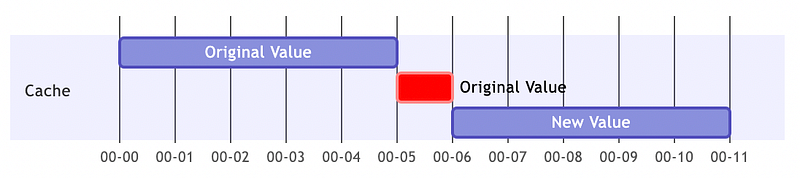
In the time interval 0–5, reading the cache will get the original value. If someone reads during the time interval 5–6, although the cache expires, the cache will be extended, so the original value will still be available. But at the same time, the first person who reads in the interval 5–6 must be responsible for updating the cache, so after the time point 6, the cache will be updated to the new value.
Let’s use a sequential diagram to represent the two concurrent request scenarios.
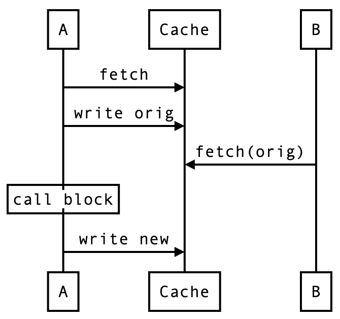
Suppose the cache has already timed out. When A fetches, it finds that the cache has timed out, so it first writes the original value back to the cache and performs the regular read operation to fetch the value from the database, and finally writes the new value back to the cache.
However, B finds that the cache has not expired when it reads, because the cache is extended, so it can get the original value.
With this approach, only one of the N concurrent requests needs to access the backend, and the rest of the N - 1 requests can still fetch the value from the cache.
Actually, Ruby on Rails’s race_condition_ttl is this implementation. Lines 855 and 856 in the link above are the operations that extend the cache time.
This approach looks like an effective way to handle high volume traffic, with only one request for access to the backend, right?
The answer is, no, not really.
This is obviously useless when facing a high-concurrency scenario. Let’s continue to describe the problem in a sequential diagram.
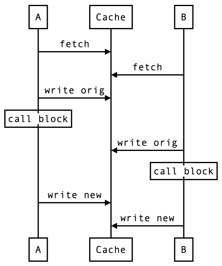
The same A and B as earlier, but this time A and B occurred very close to each other. As you can see from the sequential diagram, B has already happened when A tries to write the original value back to the cache, so B also feels he is the first one.
When N requests arrive completely at the same time, then such an implementation still cannot solve Dogpile Effect.
Exclusive lock
Extending the cache time seems to have solved most of the problems, but it’s still not good enough in a high-concurrency system. Therefore, we need a way to serialize the high-concurrency scenario. Previously, we introduced the concept of the exclusive lock.
In this approach, we are trying to avoid multiple concurrent requests to go through the cache by exclusive lock.
First, an exclusive lock must be acquired before the cache can be updated. Only those who can acquire the lock are eligible to update the cache, i. e. access the database, while the rest of the people who do not acquire the lock must wait for one of the following two conditions.
whether the cache has been updated
whether the lock can be acquired
The wait-and-acquire lock must also verify whether the cache has been updated in order to further avoid duplicate database accesses.
Of course, there is an obvious drawback to this approach. Making the concurrent process serializable would significantly reduce concurrency. In addition, the waiting is an extra overhead that not only consumes resources but also affects performance.
It’s worth mentioning that we often say Redis is not reliable, so in this scenario, is it necessary to use Redlock to further improve reliability?
It depends.
In general, no, even if Redis is not reliable enough to be used exactly once, the rare occurrence of a leak is not a problem in this scenario. This is not a scenario that requires strong consistency, but at best a few accesses to the database.
Conclusion
In order to address a common problem with caching, Dogpile Effect, we have reviewed three common approaches.
The scenario where the warm up cache is applicable is the “critical cache”. Once we can narrow down the scope of the cache, then keeping it fresh is the most intuitive and easy way for us.
Extending the cache time is a general-purpose approach that can effectively tackle a variety of high-volume scenarios. By providing a time buffer, the cache is allowed to serve for a long time until the cache is updated by “someone”.
Exclusive lock is a high-concurrency specialization approach. In order to avoid concurrent requests from hitting the backend system, concurrent requests are turned into sequential requests through a serializable mechanism.
Each of these three approaches has its own advantages and benefits, but in fact, extend cache time and exclusive lock can be combined into a total solution. I will explain the implementation details of this in code in the next article.
This week, in our study group, there is an interesting question.
If our service use MongoDB as the primary database and leverage ElasticSearch to benefit searching. Each request is in, our service is responsible for a dual write to update both MongoDB and ElasticSearch. Is this implementation considered CQRS?
In fact, this implementation is indeed generating a read model for searching and a write model for domain operations. If there is any search request, we can build a search layer or a search service for that.
This looks like CQRS, doesn’t it?
In my opinion, such an implementation is not CQRS.
There are two core concepts about CQRS.
event sourcing
responsibility segregation
Let’s see their actual meaning.
Event sourcing
Event sourcing is the most important concept for CQRS. When we have a new feature requirement, we can leverage the existed events and replay to generate a new read model so that we don’t need to modify the original code base.
In other words, we can easily fulfill any query requirement without impact the production functionality.
Let’s go back to the original example.
If our service keeps every input event in MongoDB so that new read models can be generated in the future, then I would say it’s “very much like” CQRS.
Responsibility segregation
The another key point is the responsibility segregation, i.e., the last two letters of CQRS.
What does that mean?
From my point of view, responsibility for building the read and write models must be separated.
If our service is responsible for both update MongoDB and update ElasticSearch, that doesn’t sound separate at all.
In order to release the burden of updating many models, CQRS introduces an event synchronization mechanism for event consumers to generate read models and make them consistent eventually.
Let’s continue with the original example.
If our service maintain the MongoDB’s domain states and keep every domain operation as audit logs. Then, we can build a worker who regularly digest these logs and update ElasticSearch. So, this is a CQRS definitely.
Conclusion
Why do we need to clarify these terminology details? Is it important to know if it is considered CQRS?
Well, it depends.
If we want to make the original system better, then we need to know exactly what a paradigm means. If we hastily assume that the original system is already a paradigm, then we miss the opportunity to look at it deeply.
The original implementation actually works well at the moment. However, if the input request increases, updating ElasticSearch will become a bottleneck while handling domain operations. At that time, we then have to make additional improvements.
Those paradigms are the indexes that provide how to improve. Because of this, we need to understand the specifics of the paradigms.
Explaining how to achieve end-to-end exactly-once guarantee
Previously, when discussing message queues, we mentioned that when selecting a message queue, we should consider its delivery guarantee. Depending on the needs, there are different requirements for the delivery guarantee. The more critical the application, the higher level of guarantee is required.
There are three different levels of delivery guarantees, ranging from weak to strong as follows.
At most once
At least once
Exactly once
When we define a delivery guarantee, in fact, we need to understand the scope of the guarantee. In an end-to-end delivery guarantee, there are three different paths that work together to define a complete end-to-end delivery guarantee.
These three paths are as follows.
Producer Perspective
Consumer Perspective
Sink Perspective
An end-to-end delivery guarantee is actually determined by the weakest of these three paths. For example, if the producer has an exactly-once guarantee, but the consumer can only achieve at-least once, and the sink has at-least once too, then end-to-end is at-least once guaranteed.
In this article, we will focus on how to achieve an exactly-once guarantee. Therefore, it is necessary to understand the meaning of these three paths and how to handle failures.
Producer Perspective
From the producer’s point of view, we always want any message that is sent to be delivered.
Most message queues are able to tell the producer whether the message was sent successfully or not, and when the message is sent successfully, the producer will receive a response. We can be sure that if we receive a response, it was successful, and if we don’t receive it, it’s basically a failure.
However, if we just lose the response but send it successfully, we have a problem.
The diagram above shows a common error process, so how do we avoid sending twice?
There are several approaches.
The first approach is for the producer to maintain a unique constraint on the message, e.g. (producer_id, msg_id). When a send failure occurs, the producer goes to the broker and queries the broker’s internal storage to determine whether the send failed or the response was lost.
Nevertheless, not every message queue supports this approach. If the message disappears as soon as it is taken away by the consumer, such as RabbitMQ, then this approach will not work. Conversely, systems like Kafka, which store messages as logs, can provide producers with queries.
In the second approach, the producer does not identify if a response is lost, instead resending the message anyway, but leaving a GUID (globally unique ID) on the message. On the other hand, the consumer receives the message and has to determine if the GUID has been processed, or simply ignore it if it has been processed.
If using Kafka, there is another approach to guarantee exactly-once, that is, through message transactions.
Just like a relational database, declare START TRANSACTION before sending a message, and declare COMMIT after the message is sent. If any of the intermediate messages fail, then the producer does not COMMIT but simply aborts the entire transaction and resends it. In this way, a failed resend does not result in a duplicate send.
Consumer Perspective
This is the scenario that all message queues focus on. The delivery guarantee provided by the message queue is only a part of the overall end-to-end delivery guarantee from the consumer perspective.
Most message queues can only provide at-least once guarantee. Once the consumer has correctly processed the message, an acknowledgment is sent to the message queue, and the message is removed only when the message queue receives the acknowledgment.
And, the flow of the problem is as follows.
When Consumer 1 handles Message A and an acknowledgment is lost, then Consumer 2 can continue to get the same Message A and handle it, resulting in handling twice.
Basically, this is a common problem for messages queues that are supported at-least once.
Idempotent Updates
In general, developers try to make messages as idempotent as possible so that they do not cause problems no matter how many times a message is handled.
As mentioned in the previous section, putting a GUID inside each message is an obvious solution. Consumers store handled messages in a durable storage, and each consumer must verify whether a message has been handled before handling it.
In addition, consumers must avoid duplicate updates when updating the storage by using transactions.
Let’s take MySQL as an example.
1 2 3 4 5
START TRANSACTION; $RET =UPDATE event SET handled =trueWHERE msg_id =123AND handled =false; if $RET ==1: Do whatever you want; COMMIT;
Please notice in the first line after the transaction, in addition to msg_id in the WHERE clause we must also add handled = false, this is one of the ways to avoid MySQL having racing conditions. If we don’t add this check condition, it is still possible to process the same message twice under race conditions.
There is a detailed explanation of how MySQL handles race conditions in my previous article, if you want to know the details you can refer to the following.
Nevertheless, it is not easy to make the message idempotent. In addition to the consumer, it often requires the cooperation of the producer, which adds to the coupling and complexity.
Event Sourcing
Another approach is to use event sourcing. To implement event sourcing, the message queue must support querying message logs, such as Kafka.
Event sourcing means that the current state of the consumer is generated by replaying all events, so any event handling failure can be recovered by simply replaying the event from the beginning.
However, this approach creates two problems.
The efficiency of replaying from scratch is not good.
It is difficult to get a list of several current states.
To solve the first problem, a checkpoint mechanism is usually used. Take snapshots of the states and record offsets at regular time intervals or for each batch of messages handled.
When a problem occurs, just restore the last snapshot and replay the last offset to the latest data. Through the checkpoint mechanism, we can greatly improve the replay efficiency.
The second problem is usually solved by using CQRS, so that a variety of different read requirements have a snapshot available for reference. For more information on how to evolve the CQRS architecture, please refer to my previous article.
To sum up, in order to achieve an exactly-once guarantee by using event sourcing, the consumer must be able to record the handled states and offsets; when each error occurs, the consumer discards the current result and tries to replay it from the previous state snapshot to get the correct result.
Sink Perspective
Sink means downstream of the message. In fact, the sink perspective is a special case of the customer perspective.
Suppose the sink is a database, the consumer itself can already achieve exactly-once guarantee through the event sourcing.
But this is not enough, because in the process of recovering the consumer will propagate the event to the next again, resulting in downstream receiving duplicate results of the same event.
In the above process, the consumer itself can guarantee exactly-once by restoring the state, but the downstream database has been written twice, which is still a problem.
Honestly, there is no silver bullet in sink that can completely achieve exactly-once guarantee without side effects.
Let’s check Solution 1, we only output the accumulated results after the consumer has successfully created a checkpoint.
Since consumers are guaranteed exactly-once through the checkpoint mechanism, we only output the results when the checkpoint is created, thus ensuring consistency between consumer and sink. It is important to make the checkpoint creation and output be transactional.
However, Solution 1 has an obvious drawback. The message handling loses its real-time nature and generates spikes in the database. Because the checkpoints are created in batches, not for each message, i.e., there are no current results in the database. In addition, the output process is also batch, which results in a large number of writes to the database at regular intervals.
So, let’s see Solution 2, which makes the database update idempotent.
It is straightforward to simply make each database update have a primary key and overwrite the rows with the same primary key.
However, Solution 2 also has drawbacks. Firstly, it is not easy to define the primary key for each update. Secondly, when a consumer fails to handle and starts a replay, the saved results may time travel and be reverted back to the past then updated again.
This inconsistency depends on how often the checkpoints are created and how efficiently they are replayed, which can take up to a couple of minutes.
Both Solution 1 and Solution 2 have their potential risks, but if I had to choose, I would prefer Solution 2 more.
Conclusion
In this article, we take a closer look at the semantics of exactly-once and understand how end-to-end exactly-once can be implemented.
Starting with the message producer at the beginning, the message is sent and enters the message queue, then is read and handled by the consumer, and finally the result is output downstream.
I have to say exactly-once guarantee is a very difficult holy grail to achieve, and it has to be done correctly at every stage of the message flow in order to fully achieve end-to-end exactly-once guarantee.
I believe there must be some original designs besides listed in this article that I have never noticed, if you have your own implementation, please feel free to share with me.