CT Wu

Software Architect · Backend · Data Engineering

Last week, we introduced how to build a PyFlink experiment environment, and today we will use that experimental environment to explore the possibilities of PyFlink.

PyFlink is a general purpose streaming framework and abstracts streaming processing into four levels.

  1. SQL
  2. Table API
  3. DataStream
  4. Stateful Stream Processing

The closer to the bottom the more flexibility is available, but also requiring writing more code. I would like to be able to do almost everything with PyFlink, so let’s get started with the basic concepts of PyFlink development from a DataStream perspective.

This article will introduce a few key points of PyFlink development with simple descriptions and examples, but will not mention the implementation details of Flink.

DataStream Concept

The development of DataStream will follow the following process.

Basically, we get streaming data from a source, process it, and output it to somewhere.

This is expressed in PyFlink as follows.

1
2
3
ds = env.add_source(kafka_consumer)  
ds = ds.map(transform, output_type=output_type_info)
ds.add_sink(kafka_producer)

Source and sink are easy to understand, but the key is what processing can be used?

In the official document there is a list of all available operations.
https://nightlies.apache.org/flink/flink-docs-release-1.15/docs/dev/datastream/operators/overview/

For the above example, we used map.

There is also an example of the operation in the Flink artifact, the code is placed at ./examples/python/datastream/basic_operations.py

What is the difference between map and flat_map?

There are two similar operations in the operation list, map and flat_map, what is the difference between these two operations?

The difference is in the number of generated outputs.

In the case of map, an input event generates one and only one output event; on the other hand, flat_map can generate zero to many output events.

Let’s use the actual code as an example.

1
2
3
4
5
6
7
8
9
def map_transform(i: int):  
return i * i

def flat_map_transform(i: int):
for idx in range(i):
yield idx

ds.map(map_transform, output_type=Types.INT())
ds.flat_map(flat_map_transform, output_type=Types.INT())

In this example, map squares all the input integers and passes them out, one input corresponds to one output. However, flat_map outputs a series of events, and the number of output events is determined by the input events.

If the input is 0, then yield of flat_map will not be triggered, and nothing will be generated.

State

State is the best feature of Flink.

Although we have various operations available, many of them actually produce results based on previous events. How do we keep the previous events? This is where State comes in.

State can be considered as an internal storage in order to persist data, and the size of State is the summary of every node’s memory.

Nevertheless, State can be persisted in a durable storage like RocksDB to gain more scalability.

1
from pyflink.datastream import StreamExecutionEnvironment, EmbeddedRocksDBStateBackend
1
2
env = StreamExecutionEnvironment.get_execution_environment()  
env.set_state_backend(EmbeddedRocksDBStateBackend())

To use State in Flink framework, there are two key points worth noting.

  1. State can only be used in “Keyed Data Stream”.
  2. State is based on operations and not able to share with others.

All available States and the reference are listing below.
https://nightlies.apache.org/flink/flink-docs-release-1.15/docs/dev/datastream/fault-tolerance/state/

In fact, an example at ./examples/python/datastream/state_access.py also provides a good demonstration.

Connect (Shared State)

As mentioned in the previous section, states are operation-based and cannot be shared, but sometimes we indeed need to combine two different streaming states, so what should we do?

Fortunately, Flink provides connect to enable us to share the states of different streams within the same job.

By using connect, we can combine different streams and use the same operation, so that we can share the same operation state.

To be more concrete, let me provide a practical example. There are two streams.

  • Stream 1 provides a mapping between the item identifiers and the item names. When the item name changes, an event (item_id, item_name) is sent into the stream, so we just need to save the latest status.
  • Stream 2 is the transaction history, including which item was sold and the number of items ordered.

What we want to do is, when any purchase is entered, then we have to sum it up and append the latest item name to it.

This is the classic streaming enrichment pattern, and I explained the enrichment design pattern in detail in my previous article.

Here is the full program example.

In flat_map1 the stream 1 is handled, that is to say, the mapping of item number and item name is maintained, so this stream does not need to generate output events.

The core of the whole application is in flat_map2. We take the accumulated quantity from self.cnt_state and not only add the new quantity but also update it back to the state. Then, in the output process, we take the corresponding name from self.state and finally we output the enriched events.

Conclusion

In the last example, we demonstrate the operation, state, and merging of streams.

From this example, we can easily understand that Flink can do anything we want as long as we write the program correctly.

We will continue to do some experiments on stream processing and will continue to publish any further updates if there are any.

Originally published on Medium

I am trying to play with PyFlink recently, but there is not much information available on the Internet, and most of the information is a bit outdated. So I’ll document how I set up the environment and actually experiment with PyFlink.

Before starting, let’s set the experiment goals.

  1. To run PyFlink instead of Flink, because I can’t code in JAVA.
  2. To run on K8s, not docker or standalone.
  3. Use the latest version of Flink, 1.15.2.

I briefly describe the entire experimental process.

  1. Create a K8s cluster.
  2. Deploy PyFlink cluster.
  3. Upload the job from the local machine.
  4. Check the job status in the dashboard.

Now, I believe you all understand the experimental process, so let’s start preparing the preconditions.

Once all is ready, let’s get started!

Create a K8s cluster

My personal preference is to use K3s to create clusters rather than minikube.

There are several reasons.

  1. It is easier to share the environment. My experimental environment is on EC2, so anyone who knows the location can use it.
  2. It is more resource efficient. minikube has high system requirements, while K3s itself is designed for IoT devices and is relatively resource efficient.
  3. K3s is a regular K8s, there are no special features.

After setting up the cluster according to the official document, some extra settings are required.

Create a namespace.

  • kubectl create ns flink

Create a service account.

  • kubectl create serviceaccount flink -n flink

Grant authorization for the service account.

  • kubectl create clusterrolebinding flink-role-bind --clusterrole=edit --serviceaccount=flink:flink

To build a PyFlink cluster we need to prepare the container image to support PyFlink first as follows.

https://hub.docker.com/r/wirelessr/pyflink

The Dockerfile to build the container is also available in Dockerhub.

Next, download the latest stable version of flink artifact locally.

https://www.apache.org/dyn/closer.lua/flink/flink-1.15.2/flink-1.15.2-bin-scala_2.12.tgz

After decompression we have to add some fat jar that is required but not packaged into it.

Download bcprov-jdk15on and bcpkix-jdk15on jar files at

Then move them to the folder

./flink-1.15.2/lib

When everything is ready, we can run the PyFlink cluster on K8s.

1
2
3
4
5
6
7
8
9
10
11
12
./bin/kubernetes-session.sh \  
-Dkubernetes.namespace=flink \
-Dkubernetes.jobmanager.service-account=flink \
-Dkubernetes.rest-service.exposed.type=NodePort \
-Dkubernetes.cluster-id=flink-cluster \
-Dkubernetes.jobmanager.cpu=0.2 \
-Djobmanager.memory.process.size=1024m \
-Dresourcemanager.taskmanager-timeout=3600000 \
-Dkubernetes.taskmanager.cpu=0.2 \
-Dtaskmanager.memory.process.size=1024m \
-Dtaskmanager.numberOfTaskSlots=1 \
-Dkubernetes.container.image=wirelessr/pyflink:1.15.2-scala_2.12-python_3.7

There are two key points noteworthy.

  1. rest-service.exposed.type=NodePort. In order to allow users to access the PyFlink cluster, and to simplify the experiment process, we choose to use NodePort as the external interface.
  2. We must specify the container.image that can support PyFlink, in this case, the Dockerhub mentioned earlier.

By using kubectl get svc -n flink we can know which port the dashboard (flink-cluster-rest) is running on. This dashboard location will also be the entry point for the jobs we want to submit later.

Submit a job

Most of the Flink examples will use examples/batch/WordCount.jar as the first Hello World.

So we can also use this Jar file to test whether Flink can run correctly.

1
2
3
./bin/flink run \  
-m ${flink-cluster-rest}:${port} \
examples/batch/WordCount.jar

After submitting, we can check the result in the dashboard, normally, it will be executed successfully. But this example is JAVA-based, so we’ll proceed with a Python-based example to verify PyFlink.

Before we start, we need to install the PyFlink package locally.

pip3 install apache-flink==1.15.2

If we are not using M1 chip, this command should install successfully without any problems.

Same as the WordCount example, Python also has a corresponding WordCount example in examples/python/table/word_count.py.

However, the Python example needs to be modified a bit to work properly. Find this comment line:

remove .wait if submitting to a remote cluster

Follow the instructions to remove the .wait above, and then we try to submit the Python job.

1
2
3
./bin/flink run \  
-m ${flink-cluster-rest}:${port} \
-py ./examples/python/table/word_count.py

Returning to the dashboard should show the job is also performing properly.

Conclusion

There is very little information about PyFLink, both in terms of environment installation and coding reference, so I hope this article will be helpful to you.

However, this article does not explain the details of Flink cluster and how to develop PyFlink in detail, I’ll leave those details for a future article.

Originally published on Medium

Building Apache Pinot and Presto

Working on streaming database step by step

Recently, we have been surveying some streaming database solutions and the primary target is Apache Pinot, which fits our needs from the description and is therefore the primary target.

Apache Pinot, a real-time distributed OLAP datastore, purpose-built for low-latency high throughput analytics, perfect for user-facing analytical workloads.

However, some of the official documents are actually missing, so I found some information on the Internet and finally was able to do some experiments. These processes were not documented at that time, so I am not sure what reference materials were actually used.

Currently, the entire experimental infrastructure is built with docker-compose, and the complete codes in Github repository is as follows.
https://github.com/wirelessr/pinot-plus-presto

Apache Pinot

To explain the core components first, let’s take a look at docker-compose.yml.

1
2
3
4
5
6
7
8
9
10
11
12
13
14
15
16
17
18
19
20
21
22
23
24
25
26
27
services:  
zookeeper:
image: zookeeper:3.5.6

pinot-controller:
image: apachepinot/pinot:0.9.3
ports:
- "9000:9000"
- "8888"
environment:
JAVA_OPTS: "-javaagent:/opt/pinot/etc/jmx_prometheus_javaagent/jmx_prometheus_javaagent-0.12.0.jar=8888:/opt/pinot/etc/jmx_prometheus_javaagent/configs/pinot.yml -Dplugins.dir=/opt/pinot/plugins -Xms1G -Xmx4G -XX:+UseG1GC -XX:MaxGCPauseMillis=200 -Xloggc:gc-pinot-controller.log"

pinot-broker:
image: apachepinot/pinot:0.9.3
ports:
- "8099:8099"
- "8888"
environment:
JAVA_OPTS: "-javaagent:/opt/pinot/etc/jmx_prometheus_javaagent/jmx_prometheus_javaagent-0.12.0.jar=8888:/opt/pinot/etc/jmx_prometheus_javaagent/configs/pinot.yml -Dplugins.dir=/opt/pinot/plugins -Xms4G -Xmx4G -XX:+UseG1GC -XX:MaxGCPauseMillis=200 -Xloggc:gc-pinot-broker.log"

pinot-server:
image: apachepinot/pinot:0.9.3
ports:
- "8098:8098"
- "8888"
environment:
JAVA_OPTS: "-javaagent:/opt/pinot/etc/jmx_prometheus_javaagent/jmx_prometheus_javaagent-0.12.0.jar=8888:/opt/pinot/etc/jmx_prometheus_javaagent/configs/pinot.yml -Dplugins.dir=/opt/pinot/plugins -Xms4G -Xmx16G -XX:+UseG1GC -XX:MaxGCPauseMillis=200 -Xloggc:gc-pinot-server.log"

The above are the four basic services needed to construct a Pinot, most of the same as the official document are omitted and only the parts I modified are listed. By the way, I have changed the image version to the new one, but let’s keep the official version in the example.

The main changes are to the ports and environment of the three Pinot services, in order to make Pinot’s metrics available by Prometheus.

Therefore, ports opens an additional 8888 and adds an additional javaagent parameter to JAVA_OPTS. The purpose of the javaagent is to enable the original Pinot JMX metrics to be web-based and exposed to Prometheus.

So far, the jmx_prometheus_javaagent.jar in the official document does not include the version number, but I could not find the corresponding file from the official container, so I have to use the jmx_prometheus_javaagent-0.12.0.jar instead.

Monitoring

In order to observe the state of the services, we also need to build Prometheus and Grafana.

1
2
3
4
5
6
7
8
9
10
11
12
13
14
15
16
17
18
19
prometheus:  
image: prom/prometheus
container_name: monitoring-prometheus
restart: unless-stopped
volumes:
- monitoring-prometheus-data-1:/prometheus
- ./volumes/prometheus/prometheus.yml:/etc/prometheus/prometheus.yml
ports:
- "9090:9090"
grafana:
image: grafana/grafana
volumes:
- ./volumes/grafana/provisioning:/etc/grafana/provisioning
- ./volumes/grafana/dashboards:/var/lib/grafana/dashboards
ports:
- "3000:3000"
environment:
GF_SERVER_ROOT_URL: https://localhost:3000
GF_SECURITY_ADMIN_PASSWORD: password

In volumes we define the required configuration files for these two services.

  • Prometheus needs to know where to fetch the metrics from, so it needs to set the FQDNs of the three Pinot services.
  • Grafana requires data source settings and a Pinot-specific dashboard.

After running docker-compose, we can view the dashboard from https://localhost:3000. The account and password are simply admin and password.

Apache Presto

The last service is Presto.

Why do we need Presto? Because Pinot supports SQL, but in fact Pinot does not support JOIN. If there is a need to merge two tables, it must be provided by an external SQL engine.

Presto is a SQL engine that supports ANSI SQL and multiple data sources, including Pinot of course, so I chose to use Presto in my experiment.

1
2
3
4
5
presto-coordinator:  
image: apachepinot/pinot-presto
restart: unless-stopped
ports:
- "18080:8080"

Presto has two roles, coordinator and worker. In the experimental environment, we simply use the built-in worker of the coordinator.

The official container apachepinot/pinot-presto is the coordinator by default without any settings, and already uses the FQDN pinot-controller:9000, so there is no need to change anything, we can use it directly.

Conclusion

After cloning the Github repository, we can run docker-compose up -d directly to get the experimental environment up and running well.

The whole experimental environment contains three key points.

  1. Apache Pinot: the streaming database itself.
  2. Prometheus and Grafana: the monitoring system that emulates the production environment.
  3. Apache Presto: a query capability that is not available in Pinot.

By the way, the official document does not introduce how to use Kafka with security, only Kafka without security as an example.

In the case of Confluent, Kafka has built-in SASL_SSL, I refer to this article to set up Kafka’s account and password.
https://dev.startree.ai/docs/pinot/recipes/kafka-sasl

This experimental environment may be expanded for some of my needs, such as adding Presto workers.

Originally published on Medium

Start from a small step

Last time we talked about the evolution of the data infrastructure, the whole evolution process is as follows.

  • Stage 0: None
  • Stage 1: Batching
  • Stage 2: Streaming
  • Stage 3: Integrated
  • Stage 4: Automation
  • Stage 5: Decentralization

But remember? The evolution from stage 1 to stage 2 was a bit weird in that we just dropped the batch processing we were using and built a new stream processing.

In fact, a product that is already on production environment not make such a drastic change, but would choose an incremental migration process instead.

Therefore, in this article, we will explain in detail how the migration from stage 1 to stage 2 will work in practice.

Stage 1: Batching

Let’s review the batch architecture again.

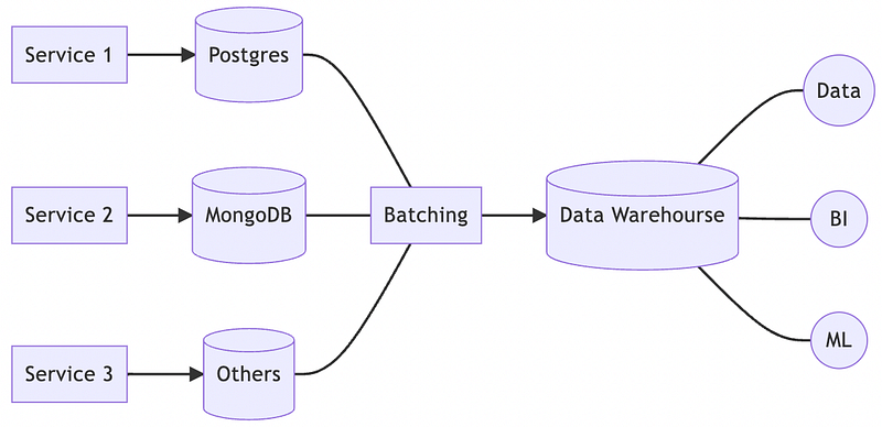
Under this architecture, we have a batch processing role responsible for archiving data from various services to the data warehouse. And batch processing also performs data pre-processing to generate structured data for accelerated analysis purposes.

However, in order to support real-time analytics, we knew from the previous article that we had to introduce a streaming architecture, but at the same time we wanted to leave the original analytics functionality as is.

In other words, it was necessary to add additional real-time analytics capabilities while maintaining the existing architecture and functionality.

So, let’s start trying to add streaming architecture.

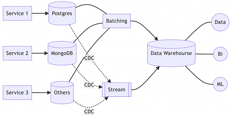
Stage 1.5: Batching + Streaming

In the previous article, we took an aggressive approach by simply dropping batch processing and replacing it with streaming. This would make the architecture simple, but comes at the cost of a complete rewrite of all the analysis, since the data from streaming is not in the same format as the data from batch processing.

Therefore, we add an extra 1.5 stage to allow batch and streaming to coexist for a while until we could change the analysis framework to use streaming data sources for all subsequent analyses.

The advantage of this is of course that we don’t need to do a Big Bang.

As Martin Fowler reportedly said, “the only thing a Big Bang rewrite guarantees is a Big Bang!”.

However, the drawback is obvious, when there is any requirement for modification, we have to implement both batch processing and streaming processing, which greatly increases the difficulty of maintenance.

Therefore, although there is a 1.5 stage, it is important to realize that this is only a transition period and should not be considered as a solution.

Stage 2: Streaming

Once we have a transition period, we can evolve more smoothly from batch processing to streaming processing. In the previous stage, we will gradually move all the functionality from batch processing to streaming processing.

At the end, it’s just easier to take away the batch processing.

But as I stated in my previous article, batch processing still has its value, so even if it is taken out of the main data pipeline, we will still have batch processing there.

It will just change from being the primary data producer to a secondary one, regularly reorganizing the data in the data warehouse to improve data utilization. Of course, batch processing can also be used to move out-of-date data from the data warehouse to cold storage, further saving storage costs.

Conclusion

The whole evolutionary process should be smooth and gradual.

In order to avoid a Big Bang, it is a difficult choice to move from one architecture to another. Each migration should have as small impact as possible, but at the same time, it should not be too small to make the pain period too long.

Overall, every organization has a different tempo. For an organization with sufficient human resources, this forward movement can be aggressive and fast, or on the contrary, measured.

But in any case, it is important to understand the dilemma and come up with a reasonable enough approach and, more importantly, a complete migration plan.

This planning process is actually as important as the architecture change.

Originally published on Medium

From Monolith to Self-service Platform

All systems start as a small monolith. In the beginning, when resources and manpower are not sufficient, the monolith is the choice we have to make, even the data infrastructure is no exception.

But as requirements increase, there are more and more scenarios that cannot be achieved by the current architecture, and the system must therefore evolve. Each time the system evolves, it is to solve the problems encountered, so it is necessary to understand the different aspects that need to be considered, and to use the most efficient engineering methods to achieve the goal.

In this article, we will still start with a monolith, as we have done before.

But this time, our goal is not to serve a production environment, but to provide the data infrastructure behind all production environments.

A data infrastructure is a “place” where all kinds of data are stored, either structured data or time series data or even raw data. The purpose of this big data (and they are really big) is to provide material for data analysis, business intelligence or machine learning.

In addition to internal uses, there may also be user-facing functions, for example, a list of recommended products on an e-commerce website. The recommendation function is the most commonly used customer scenario for big data, such as recommended products in e-commerce websites and recommended videos in video platforms like Youtube. All of these are the result of analyzing, aggregating, and compiling after storing various user actions.

After knowing today’s topic, let’s get to work.

Monolithic architecture

Let’s begin with a monolithic architecture.
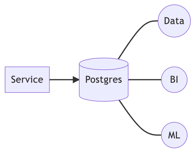
Whatever the service is, a typical monolithic architecture is a service paired with a database. All data analysis, business intelligence and machine learning run directly on this database.

This is the simplest practice, but it is also the beginning of all products.

Why do we show it in monolithic style? Wouldn’t it be better to do more?

Well, if the product dies before it is popular, then the monolith will be enough to maintain full features. In order to avoid over-engineering and the investment cost getting exploded, we prefer to start with the easiest proof-of-concept monoliths.

Of course, this architecture is sure to encounter problems. There are three common problems.

  1. The analysis affects the production performance.
  2. If the microservices are introduced, running analysis on each microservice’s database is suffered.
  3. It is very difficult to perform cross-service analysis.

Various analyses inevitably take up a lot of database resources, so customers directly feel the poor performance during that time.

In addition, when product requirements increase, we usually adopt microservices for rapid iteration, which means many service and database pairings are created. In order to be able to analyze various product requirements, it is necessary to build several analysis frameworks on every database.

Moreover, even if each service can be analyzed individually, we cannot easily obtain a global view because the analytics are independent of each other.

Therefore it is necessary to perform the first evolution.

Batch processing

We have two goals, firstly to have independent data storage so it does not directly affect the production environment, and secondly to be able to perform cross-service analysis.
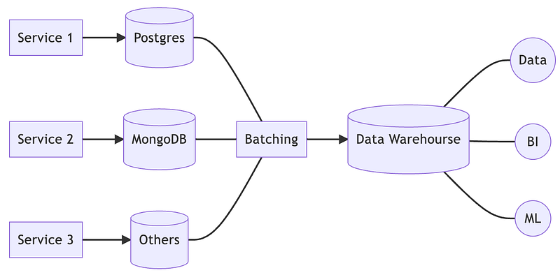
To achieve these goals, we set up a centralized data warehouse so that all data can be stored in one place. All analyses were migrated from the databases of each service to the data warehouse.

We also need a batch processing role to collect data and even pre-process data periodically so that the data warehouse contains not only raw data but also structured data to speed up the analysis.

For batch processing, I recommend using Apache Airflow, which is easy to manage and easy to script for various DAGs to address the needs of multiple batch processing scenarios.

Such an architecture is simple but powerful enough to handle a wide range of analysis and reporting scenarios. Nevertheless, there are two drawbacks that cannot be easily solved.

  1. lack of real time
  2. lack of schema

Due to the periodic batch tasks, we can’t do real-time analysis. If we run the task once an hour, then the data we see in the data warehouse is a snapshot of the previous hour’s data.

In addition, batch tasks require knowledge of the data schema of each service in order to get the data correctly and save it to the corresponding warehouse table. Assuming our data warehouse is GCP BigQuery, the schema in the warehouse table also needs to be created and modified manually.

When the number of services is very large, just knowing the schema can take a lot of time, not to mention managing it.

So, let’s do a second evolution.

Stream processing

To solve the real-time problem, the most straightforward idea is to use a streaming architecture.
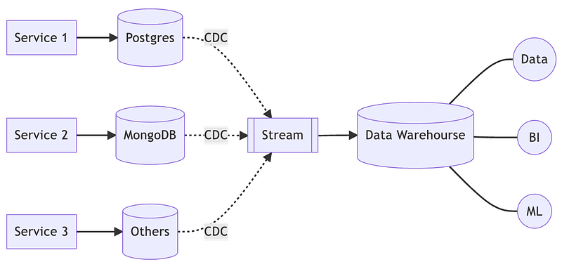
First, all the database changes of the service are captured, then the changes are sent to the stream, and finally the stream is archived to the warehouse.

But is there a way to solve the schema problem? The answer is, yes, through KCBQ.

Let’s take a closer look at the internal architecture of streaming.
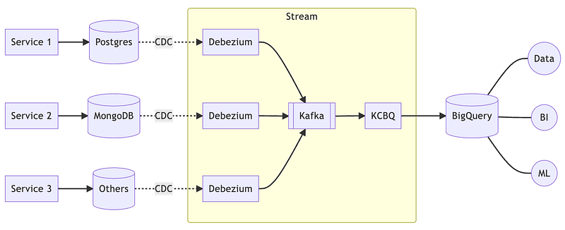
We use Debezium to capture changes to each database and send the streams to Kafka, and later KCBQ subscribes to the Kafka streams and archives them to BigQuery.

It is worth noting that KCBQ can automatically update the internal schema of BigQuery (setting needs to be enabled, and AVRO format must be used).

At this stage, we have a complete data set for analysis, and we have enough data to process for all kinds of data analysis, both real time and batch. However, in the previous stage, we were able to accelerate the analysis by batching pre-processing to generate structured data, and we still want to retain this capability.

In addition, although the data analysis is working properly, we are currently unable to support external customers to access the data. The main reason is the slow response time of data warehouse, which is a big problem when we need to interact with external customers. For example, if a recommendation list takes 5 minutes to be generated, the effectiveness of the recommendation will be close to zero.

Furthermore, when the number of features to be provided to external customers increases, data warehouse can be difficult to handle. For example, search is a common feature, but the search performance of data warehouse is very poor.

Therefore, we have to integrate batch processing and streaming processing so that this data infrastructure can flexibly support various customer-oriented functions.

Integrated architecture

We already have a batch architecture and a streaming architecture, now let’s integrate them properly.
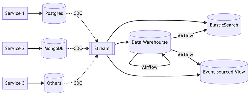
We still archive the changes from each database to the data warehouse through streaming, but we periodically use batch processing to pre-process the raw data for data analysis.

At the same time, the streaming framework not only archives, but also aggregates the streams to generate real-time customer-facing data storage. For example, ElasticSearch is often used in search contexts, while the event-sourced view is used to provide customer-facing functions, e.g., recommendation lists.

But these functions usually also require fact tables, which can be migrated from data warehouses if they are static, otherwise, they need to be implemented through stream enrichment.

So let’s further have a look at the internals of streaming architecture.
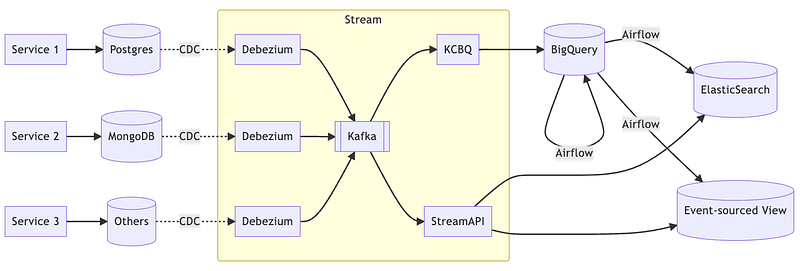
The framework is basically the same as the previous one, but with a new role, StreamAPI.

There is no specific framework specified in StreamAPI, even if using Kafka’s native library is fine.

But if using the stream processing framework can save a lot of implementation efforts, such as data partitioning, fault tolerance, state persistence, and so on.

Therefore, I still recommend using a streaming framework such as Apache Flink or Apache Kafka Streams.

At this point, the entire data infrastructure is fully functional. Whether it is for internal data analysis or for external customers, this framework can meet the requirements.

However, this architecture doesn’t mean that it’s done once and for all.

The next problem is the management problem. So far, the most common task we need to do is not feature development, but the configuration and operation of so many middleware. For each new service, we need to build Debezium, add Kafka topic, configure the streaming framework, and determine the final sink. This process also applies to a new feature request.

In addition, managing the permissions between all data stores is also a problem. When a new person comes into the organization, each participant in the framework has to grant some permissions. Similarly, when a new service or feature is launched, the permissions between services need to be managed.

What’s more, when all the data is dumped into the data warehouse, we have to encrypt or mask the PII (personally identifiable information) to be compliant with legal requirements, such as GDPR.

These tasks rely on a lot of manual work or semi-automatic scripts, which undoubtedly add a heavy load to a busy organization.

Automation (Self-service Platform)

Therefore, it is necessary to establish a fully automated mechanism to solve all management issues of the data infrastructure.
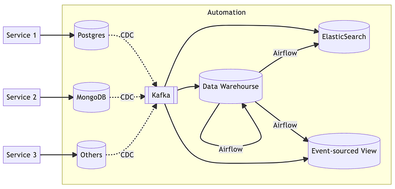
Of course, this automation mechanism should ideally be self-service, and the most successful example I have seen is Netflix’s Keystone.

This automation platform involves very deep technical details, not an article can simply explain, so I only provide the features of this platform should have, as for the implementation details will depend on the practice of each organization.

At the infrastructure level, in order to automate the establishment of settings and monitoring, it is necessary to achieve fully automated deployment through IaC (Infrastructure as Code).

In order to address the issue of data ownership, there are three permission-related controls that should also be included in the IaC as follows.

  • Identity Access Management, IAM
  • Role Based Access Control, RBAC
  • Access Control List, ACL

Privacy issues require an easy-to-use interface that can be configured to determine what data must be masked. Data Loss Prevention, aka DLP, is also a very popular data privacy topic nowadays.

As you can see from the above description, there are a lot of implementation details to achieve a fully automated management platform, and there are no shortcuts — implementation, implementation and lots of implementation.

Conclusion

This article is about the evolution of a monolithic architecture into a fully automated and fully functional data platform through continuous problem solving.

However, there are still a lot of detailed technical selections in the evolution process, such as what data storage to use, what batch processing, and what real-time processing are all worthy of attention.

Such an evolution requires a lot of human resources and time, so it is unlikely to be achieved in one step. If and only if we encounter a problem that cannot be solved, we will be forced to move to the next stage.

In fact, even if we achieve an automated platform, the evolution is still not over.

When all kinds of business requirements and all kinds of products and services have to rely on a single data engineer department, then human resources will encounter a bottleneck. How to solve it?

Since we have a fully automated management platform, we can let each product department maintain its own data warehouse and data pipeline. The data engineer becomes the provider of the platform solution, not the owner of the data.

The Data Mesh is born.

However, there are many different approaches to the Data Mesh implementation, and there is no one-size-fits-all architecture pattern.

This is all about the evolution of data infrastructure. If you have any special practices, please feel free to share them with me.

Originally published on Medium

Archiving MongoDB Changes to AWS S3

Understanding Hot-Cold Separation

In this article, we are going to introduce how to archive the audit logs stored in MongoDB to AWS S3, but before we start, let’s understand why we need it and the meaning of the need.

Audit logs are records of user actions on the system, including signing in and out, modifying data, enabling a feature, and so on. These records are kept as part of the system security, and recent data is made available for users to view. Users may be interested in the last three months of related operations, but not in records older than that.

Therefore, data that is older than three months is classified as hot data, while data that is older than three months gradually becomes warmer, i.e., rarely accessed, perhaps sometimes still. Data older than six months will be completely cold and will not be accessed except for data analysis and internal system auditing, and users will not care about the existence of such data.

That is to say, if these cold data are still in the original database, it will consume a lot of resources, including hard disk space and indexes. So, we need a way to archive these data to a lower cost storage space, but we still need to make the cold data directly available when they are to be analyzed, instead of doing further migration.

So, today’s title tells you that we will archive the data in MongoDB to AWS S3.

There are several advantages to S3, first of all, the data in AWS S3 can be easily analyzed and SQL-compatible queries can be performed through AWS Athena.

In addition, S3 is also a storage option supported by many data analytics platforms, such as Apache Spark.

Furthermore, storage cost of S3 is very low. Moreover, if it is determined that the data in S3 is for preservation purposes only and not for query purposes, it can be easily transferred to much lower cost storage, such as AWS Glacier.

Hot-Cold Separation on MongoDB

Now let’s review the requirement again.

In order to reduce the storage cost, we need to move the past audit logs from MongoDB to AWS S3. In addition, we want this to be fully automated, and I don’t believe anyone wants to manually migrate data periodically.

So what’s the best way to do this? Yes, through streaming.

We have three things to do.

  1. Pass the events from the new audit log through MongoDB’s CDC (and ignore the delete events).
  2. The stream processor archives the stream events into AWS S3.
  3. Use MongoDB’s TTL index to automatically delete expired data when adding audit logs.

By the way, the MongoDB mentioned here is not a self-hosted database, but a managed platform through Atlas. However, the same approach still applies to self-hosted databases, just with a little more setup and implementation than the managed platform.

After knowing what to do, let’s work out a solution.

Approach Details

Then, let’s explain the whole solution in detail and provide some key points worth discussing.

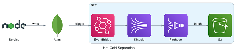
The front services and databases are original to the architecture, only the back of the streaming chain is new. The entire chain ends with our destination, AWS S3.

The first thing to do is to turn on Atlas’ built-in feature, EventBridge Triggers, and since it is a built-in feature, it only requires a few simple settings following the official documentation. There are a few key points to note here, first we only need to send INSERT events, and we need to turn on the option to send full documents so that we can save the complete audit data.

Next, we need to add a new rule to EventBridge’s third-party rules: all incoming events are sent to Kinesis, so that the source of the stream is established.

In order to fully automate S3 archiving and save transmission costs as much as possible, we add Kinesis Firehose as the stream aggregator in the middle of Kinesis and S3. Through Firehose, we can aggregate a stream of events into a batch, and write to S3 in a batch process to save S3’s transmission cost.

In this way, a fully automatic archiving is accomplished. All audit logs written to MongoDB will be archived into AWS S3 through streams.

Let’s discuss a few topics.

Why not just let the service write S3 directly?

There are two reasons.

The first is that we can achieve the purpose without changing the original application by such modification.

The other reason is that audit logs usually require transactional consistency, and it is difficult to ensure that MongoDB and AWS S3 are consistent when the primary database is MongoDB. What if writing MongoDB succeeds, but writing S3 fails?

Why Kinesis and Firehose?

In fact, we can retain one of them, if we want to keep only one I propose to keep Firehose, because we can reduce transmission costs through batch processing.

But Kinesis has a benefit, if we later want to introduce event-driven architecture or streaming processing architecture, Kinesis can provide a very good extensibility.

Does MongoDB’s TTL index affect database performance?

Yes, it does, but the impact is limited in this context. This is because we will only keep the data for a certain period of time, for example, three months.

Therefore, the amount of data is limited and the impact on the database is manageable.

Conclusion

Streaming can empower the scalability of the entire system design.

Whether it’s through database CDC or events from microservices, it can effectively improve system availability and decouple business logic from data. That’s why I’ve been sharing the streaming architecture for the last few weeks.

This time we experienced the convenience of streaming through the managed platform provided by AWS, a fully automated archiving system. Without the help of streaming, we would have to find a way to activate some scheduled mechanisms, such as a crontab, and get up once a day to check what audit logs needs to be moved, and to do large-scale data migration.

If we use such a batch design, we will immediately encounter a problem, lack of real time. When we do data migration through periodic tasks, there is a data lag, for example, one day. Any data analysis performed on S3 will not get immediate results, but rather a snapshot of some point in time in the past, which is the biggest problem with batching.

But we haven’t actually introduced some of the famous streaming framework yet, so maybe we’ll have a chance to do that in the future, but rather than actually operating streaming, I feel I’d share some more topics related to architecture and system design.

Originally published on Medium

Reducing Database Loading

Three approaches to improve database elasticity

Last week we talked about the difference between scalability and elasticity, and the concept of solutions was mentioned at a high level. In this article, let’s take a look at some practical solutions.

First, if you haven’t read the last article, I suggest you read it first. This time we are solving the elasticity problem rather than scalability. As mentioned before, the two most common solutions to the elasticity problem are caching and messaging.

Therefore, in this article, we will list some common practical solutions and briefly analyze the advantages and disadvantages. Let’s get started.

Read-aside Cache

When talking about caching, the most commonly used mechanism is the read-aside cache.

The advantage is that it is very easy to understand and implement, and already provides a good consistency level. I’ve explained how it works in my previous article, but let’s review it again.

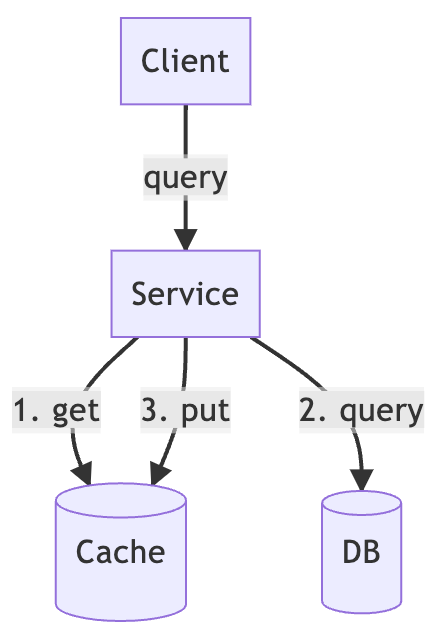
The read mechanism of the read-aside cache is very simple: first try to get the data from the cache, and if you cannot get it, then get it from the database instead, and save it back to the cache. In this way, the next request for the same data can be taken directly from the cache.

How to ensure that the cached data is up-to-date (consistency)?

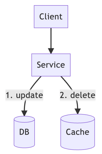
After updating the database, the corresponding records of the cache should be cleared immediately. When the same request comes in next time, it will be taken from the database first and the latest result will be written back to the cache.

It looks like both read and write are perfect, so the read-aside cache should have a high degree of consistency! In fact, not really.

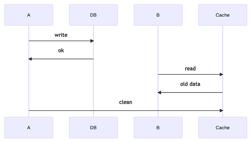
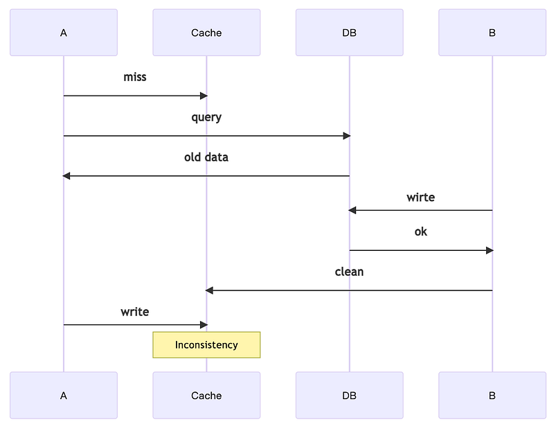
According to the above sequential diagram, we can find that both A and B are behaving correctly, but put together, they make an error, and B gets inconsistent data. This is the first problem.

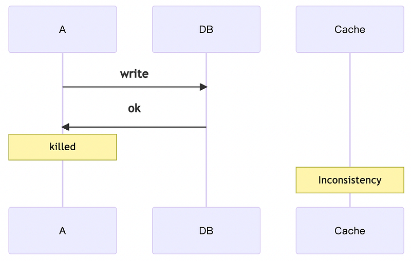
The second type of error is more intuitive, when A wants to update the data, A is killed after finishing the database update, probably due to bugs or application upgrade and so on. Then the data in the cache will remain inconsistent for a long time, until the next update or timeout.

The third error is similar to the first one in that the individual actions of A and B are correct, but put together they are wrong. This inconsistent cache data will also remain for a while until the next update.

These details have been explained in my previous article, if you want to know more can also be used as a reference.

In fact, problems 1 and 3 can be greatly mitigated by modifying the implementation of the application. In the first problem, when A finished writing the data, don’t do anything else, then clean up the cache quickly to reduce the possibility of being touched by B.

The same is true for problem 3. When A finishes querying, don’t do too much processing and write back the cache as soon as possible, which can also greatly reduce the chance of occurring after B.

However, there are three potential problems with read-aside caching.

  1. If a cache has a large scope of content, it can be difficult to determine when to clean it and to implement it. On the other hand, when many places have to be cleaned up, it may make the cache less effective.
  2. Dog pile effect. This refers to when a high-traffic system accesses cache frequently, if it encounters clearing cache or cache expiration, these traffic will still occur on the database. And the database may not be able to hold up.
  3. No graceful shutdown. Problems 1 and 3 can be improved by modifying the application, but problem 2 is not always possible, especially when the application fails, there is basically nothing to do.

Denormalization

If we have to take data from many places, it is ideal to put it all together and take it only once.

Conventionally, in order to avoid data duplication in RDBMS, we would create individual tables according to the data type, and then join each other through foreign keys.

But this will cause a problem, if it is an aggregated data must be pulled from each table, in the traffic and data volume of the system is not large, this approach is reasonable, and will have good performance. However, in a big data scenario, such performance is tragic.

The performance of JOIN is not good enough for large data, and it is even worse if it is a subquery.

Therefore, the idea of denormalization is to put all the data together and pull all the required data through a single query. Common practices include Facts Tables, etc., but this article does not focus on data modeling, but on system architecture.

However, the problem is that reading from one place is possible, but what about writing to it? The original tables are already in use by clients, so do we need to find all the clients to modify them? No, it’s too much work!

There are two ways, synchronization and asynchronization.

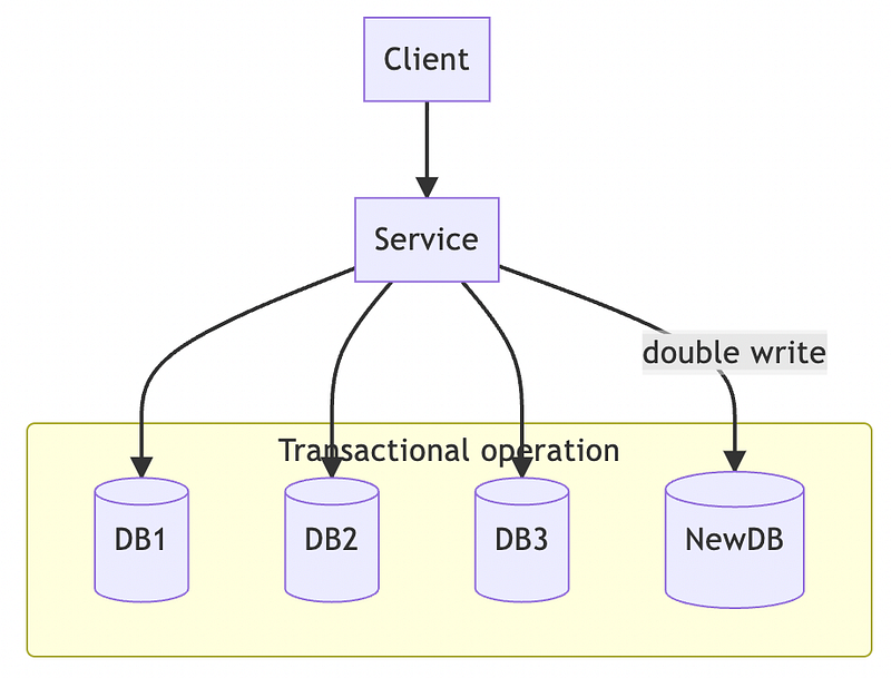
This is an architecture of synchronization. The following DBs can be treated as databases or tables or even caches.

When the service needs to write data, originally only DB1, DB2 and DB3 need to be written, in order to achieve denormalization, but also need to write NewDB in code, and NewDB is the result of aggregation.

If someone needs to aggregate results, they can pull them directly from NewDB. If the owners of these DBs all belong to the same functional team, then this implementation looks acceptable.

On the contrary, if the team that needs to consolidate the results is another functional team, such an architecture will not work. First, the other functional team has to find all the updates, then they have to make changes within the service, and they have to do it transactionally.

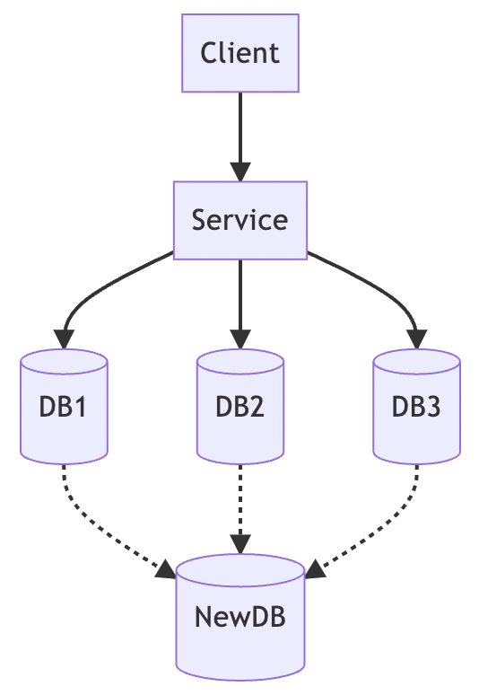
For a cross-functional team, such a workflow is unrealistic and impossible. Hence, asynchronous data replication is introduced.

This architecture should be very common in my previous articles, it is in fact CQRS.

Nevertheless, there are various practices to implement CQRS, some of which are listed below. The following is a list of common practices from long to short time intervals.

ETL

DBs -> Batching -> Materialized View

This is the most common practice nowadays, and almost all data engineers do it this way. Data is migrated from one place to another through batch processing, whether it is Hadoop or Spark.

Some transformations and business logic may be added in the process. In order to make the data more accessible, if RDBMS is used as the NewDB, then Materialized View may be added. The data is snapshotted by predefined rules, and if the data is updated, it is refreshed to respond to the calculation of new data.

But data migration is a very costly practice, so ETL does not happen all the time, instead, it happens once an hour or even once a day.

Therefore, the data obtained from NewDB will not be the latest, but a snapshot at a certain point in time.

CDC

In order to keep the data as up-to-date as possible, we know that ETL is not enough. Therefore, CDC is another common practice.

DBs -> Debezium -> Kafka -> Streaming DB

When data is updated, it is captured by Debezium, streamed out to Kafka, and finally written to a streaming database.

The streaming database is made available to external users, so the streaming database must be able to support not only streaming writes, but also rapid query capabilities.

There are many mainstream streaming databases, and Apache Pinot is the most popular one recently.

Because CDC streams are updated in real time, external users can get almost real-time data.

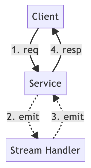
Streaming

Another mechanism for real time streaming comes from the service that originally wrote the data.

Service -> Kafka -> Stream Handler -> RocksDB

When the service finishes updating the original database, it actively sends an event to Kafka and Kafka dispatches it.

In such a system, it is most common to use a streaming framework to do the pre-processing of the streams and store them in the database. Common streaming frameworks include Apache Flink or Apache Samza, and of course the recent Kafka Stream.

For the backend database, we choose a state persistence mechanism that can match the streaming processing framework, and RocksDB is the best choice for several common streaming processing frameworks.

In this way, we can also get the latest data, but from the query point of view, the query capability provided by the streaming processing framework is not comparable to streaming database.

The above three are common data replication methods, and it is worth mentioning that the components of each method can be exchanged or even extended to each other, so that different architectures can be built based on requirements.

However, there are potential problems with asynchronous data replication.

  1. If there is a wide range of data to be used, it is a big problem to define the data to be replicated. Just as it is difficult to determine the cleanup time for a read-aside cache, it is difficult to define the scope of data replication.
  2. In addition, whether it is pre-processing through streaming framework or defining query through streaming database, the complexity is obviously high when it comes to complex data structure and complicated computation.
  3. Among these three methods, ETL has the lowest complexity, but ETL loses data real-time.

Asynchronous requests/responses

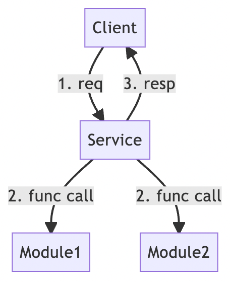
We all know the traditional request/response model as follows.

Although this is a function call here, it can also be a remote call across services.

After the client sends a request, the server responds to the request through a series of processing, which is the traditional approach. How can we do this asynchronously?

The answer is to make the implementation of the function behind the server asynchronous.

What are the benefits of doing this?

  1. Handle events by using event handlers, then we can control the number of handlers to determine the pressure on the backend system or database. In the synchronization model, when a large number of client requests come in, the server will fork threads accordingly and put pressure on the backend system. However, when the number of event handlers is controllable, the pressure on the backend system can be controlled as well.
  2. Request dedup. Since all requests from clients are entered into the message queue, event handlers have the ability to perform deduplication according to specific rules.
  3. Further, if a streaming framework is used, then the third approach from the previous section can be followed to achieve further denormalization.

However, such an architecture also has drawbacks.

  1. Such an architecture must be based on the assumption that users will refresh the page a lot in a short period of time in order to be able to play the benefits of dedup. This architecture does not mean that it is only applicable to this context, but if there is no matching context, then the implementation will be too much pain and too little gain.
  2. Implementation overhead. The server must have the ability to wait for asynchronous messages, which is simple to say, but there are many aspects of the implementation. For example, should we use a temporary queue or a permanent queue? How long should I wait? Questions like these need to be carefully considered.
  3. Starvation. In order to control the number of concurrent messages, we don’t enable handlers unlimitedly, but this also means that some people can’t wait for processing and time out.

Conclusion

This article describes some approaches to improve the elasticity of a database.

Unlike the approaches to improve scalability, scalability can be achieved through database-oriented approaches such as query optimization, indexing, and data sharding.

However, improving elasticity cannot be accomplished through databases alone, but must be accompanied by architectural adjustments, so this article lists some common approaches.

In fact, there are many more useful practices than that, and this article is aimed at small to medium-sized organizations. With a limited number of people and a limited budget, it is not possible to make large-scale changes, so we can only optimize on the original practices.

Nevertheless, I believe these approaches should provide good insights for further evolution of the system, after all, all methodologies are similar.

Originally published on Medium

Understanding the main difference between scalability and elasticity

In system design, there are two single words are confusing, which are scalability and elasticity. They are so similar that we don’t distinguish them correctly.

However, when we want to solve the issues caused by these two non-functional requirements individually, we need completely different approaches.

Therefore, in order to design the right approach we have to know them and recognize their properties. In this article, we will talk about what scalability and elasticity are and how to treat the symptoms.

Scalability

We often talked about horizontal scalability and vertical scalability, i. e., scale-out, and scale-up.

But what’s good and bad for scalability?

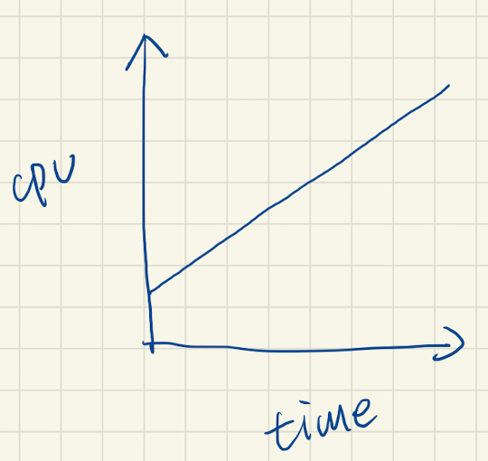
Let’s take a look at an example.

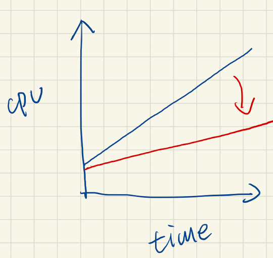
CPU grows with the time. This is normal. As the system grows, the number of users increases, the feature requirements increase, and thus the resource consumption increases as well. In this case, resources refer to CPU, but it can be applied to other resources, such as memory, response time, etc.

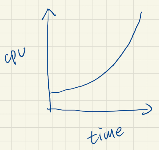
So, if this diagram indicates a normal situation, what diagram indicates a problem?

When resource usage does not rise linearly, but exponentially, something is wrong. It could be a bottleneck in usage that results in additional overhead, or a dramatic drop in performance when the amount of data exceeds a certain amount.

On the other hand, what kind of shape represents good scalability?

Similarly, resource usage rises over time, but the rate of increase shrinks, which means that scalability becomes better. The ideal state is a horizontal line, where the resource usage remains constant regardless of the number of users and the increase in feature requirements.

In other words, how to make this line as straight and as close to the horizontal as possible is the issue to be addressed in solving the scalability.

Elasticity

After talking about scalability, let’s look at an example of elasticity.

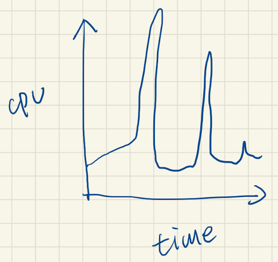
First, let’s also look at the normal situation of a system.

Resource usage fluctuates dramatically over time, with spikes occurring at certain times. It is easy to understand why this happens. Take an e-commerce site for example, when there is a Black Friday sale or Christmas coming up, the system usage will be much higher than usual. Or a ticketing site, when a top singer is going to have a concert, will also attract a large number of people to come to grab tickets.

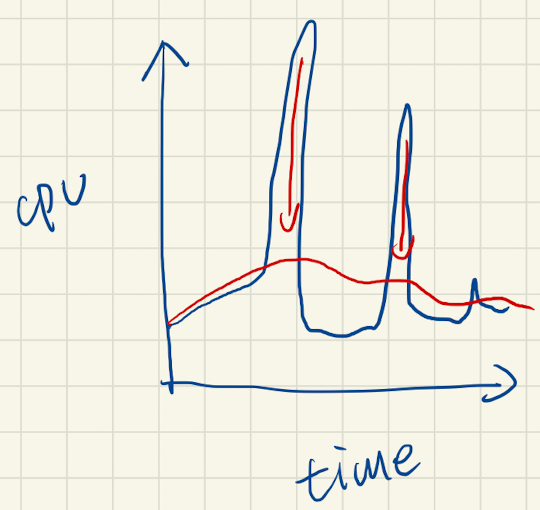
So what is good elasticity? It’s about eliminating those spikes, of course.

There are two key points in this diagram.

  1. The red line is more stable than the blue line, but the red line is not a horizontal line.
  2. The red line is significantly higher than the blue line after the occurrence of a spike.

The reason for the first point is simple, because the system usage is not fixed, so the use of resources will vary with the system usage. But in general, it can still be maintained in a stable state and there will be no significant ups and downs.

The second point, I believe, is not difficult to understand: the reason why we can flatten the blue line as much as possible is not to reject all the user requests, but to postpone the instantaneous usage through “a sort of mechanism”. Therefore, after the spike, there will always be a period of digestion, causing the red line to be higher than the blue line.

You may ask, though, the system can handle so many users without elasticity, so is it still necessary to improve the elasticity to make the effect of the red line?

The answer is, definitely. Why?

Because the highest point of the blue line is the limit of what the system can record, and more rejected user requests cannot enter the system and are not recorded. In the moment of the spike, the system’s maximum capacity is defined there, and all requests exceeding it are rejected.

On the other hand, a more elastic system has a smoother resource usage and can handle more user requests without crashing the system.

The Myth of Autoscaling

Now, we understand the scalability and elasticity. So, can you answer one question?

Ask, does autoscaling address the need for scalability or elasticity?

The answer is, scalability.

First of all, the principle of autoscaling is to track specific metrics by sampling and start scaling when the threshold is exceeded for a period of time.

Therefore, it is already a while after the spike has occurred before scaling can begin. In addition, scaling is not immediately available; even containerized applications have to go through several steps to scale, such as loading the container image and cold-starting it on a new instance. A complex application can take a few minutes from the time it decides to scale to the time it is launched.

As a result, autoscaling is not about elasticity, but about scalability.

More importantly, autoscaling does not improve the whole system. In other words, autoscaling only allows the system to continue to grow with its original scalability, but does not make it better.

One exception is that if elastic requirements can be predicted, then autoscaling can be effectively applied.

For example, if the system receives a large number of requests at the beginning of the workday (e.g., 9:00 a.m.), then the system can be autoscaled by activating it at regular intervals. In this example, setting the time of the autoscaling between 8:30 am and 9:30 am can effectively solve the elasticity problem faced during that time.

However, in general, the autoscaling faces the issue of scalability.

Conclusion

In this article, we introduced scalability and elasticity and explained what it looks like after improvement.

Nevertheless, this article does not describe how to improve scalability, because scalability is a systemic issue and there is no one specific solution that can solve it all at once.

First, bottlenecks must be identified, then the root causes must be figured out, and finally different solutions must be proposed for each bottleneck. This requires an extra investment of time and human resources to enable the system evolution, and autoscaling is a compromise to buy time. By spending additional money, the system is given time to evolve and is not shut down by the inability to scale.

But autoscaling is not a long-term solution, and additional analysis, design and implementation costs are required to fundamentally solve the scalability issue.

On the other hand, how to solve the elasticity issue?

The answer is relatively simple, through caching or messaging. In order to tolerate a large number of requests in a moment, there must be a mechanism to postpone the current spike, and the most commonly used practice is caching.

However, there are many different ways to implement caching, and the balance between caching and consistency is an important issue. I have introduced several caching practices.

  1. Consistency between Cache and Database, Part 1
  2. Consistency between Cache and Database, Part 2

These are the basic versions of caching, but there are many more advanced caching practices that will be mentioned in subsequent articles.

The purpose of this article is only to explain the two words that are easily confused, and the only way to find a feasible solution among the many approaches is to correctly understand scalability and elasticity.

Originally published on Medium

Understanding the concept of streaming architecture

Last time, we introduced streaming processing. In order to be able to handle batch and real-time data with a more pure infrastructure, we introduced Kafka and the streaming framework.

In this article, we will introduce a common design pattern for streaming, enrichment, and examine what benefits the streaming framework can bring.

What is enrichment? Briefly, it is the implementation of extending the original events to meet the new feature requirements.

Feature Description

Similar features are available on many social media platforms.

  1. Who visits me
  2. Others are also viewing
  3. What is the identity to view me

The first feature is how many people have viewed my profile in a given time period. For example, how many times my profile has been viewed in a week.

The second feature is an advanced version of the previous feature, who else did these people view? For example, 10 people viewed my profile in a week, and they also viewed Elon Musk.

The third feature is a derivative of the first one. What is the identity of these people who viewed me? For example, 10 people viewed my profile in a week, and three of them were google employees.

Who visits me & Others are also viewing

The first and second features can be easily implemented using event streaming techniques. First, let’s define a “view” event.

1
2
3
4
5
6
{  
eventType: "PageView",
timestamp: 1660270009,
viewerId: 1234,
viewedId: 5678
}

This event includes the time of occurrence and who viewed who. Then we just need to create a stream that collects all view events to analyze the features we need.

In the above diagram, suppose my user id is 4567, then it is easy to find two users who have viewed me from the event stream, which are 2345 and 1234.

Further from the stream record, we can also understand that 2345 has viewed 1234, while 1234 has viewed 5678 and 2345.

Putting this information together, we can answer.

  1. Who visits me? 2345 and 1234.
  2. Others are also viewing 1234, 5678, and 2345.

With all the event streams recorded by the streaming framework, we can perform a simple analysis to get the desired features.

What is the identity to view me?

However, it is not so simple to know what the identity to view my profile is.

Because our original event did not define additional attributes, only the id. Well, it is necessary to modify the original implementation to add new features.

Add metadata in events

Let’s add the job to the original event. When the user is viewing, in addition to sending the event with the id, the job must also be attached.

1
2
3
4
5
6
7
{  
eventType: "PageView",
timestamp: 1660270009,
viewerId: 1234,
viewedId: 5678,
viewerJob: "Google"
}

The problem seems to be solved, but is it really so?

There are several obvious issues with such a solution. Firstly, modifying the event format directly affects all downstream consumers. Under an event-driven architecture, the producer would not know the consumer’s use cases because the two are decoupled.

Secondly, events become larger, and each original event must add this new field, whether the consumer needs it or not. In other words, the overhead has gotten bigger, not just in terms of storage overhead, but also transmission overhead.

Moreover, what to do if we want to add new features? In addition to the job, the feature requires a new title, age, and so on. Then the issues mentioned above will happen again and again.

Therefore, we know this is not a good approach.

Query from external datastores

Since modifying the original event is not a good approach, we will query the required data from elsewhere as soon as we receive the event.

Although it is stated in the diagram as a database, it can also be a microservice or any platform that can provide information.

Basically, this is the most typical implementation of an event-driven architecture. When workers take events from the message queue, they process the data, either by getting the necessary information from other data sources or by storing the results in a data store, and finally by sending the enriched events to the next one.

This implementation is fine in a message queue architecture. However, in a streaming framework, such an implementation creates a performance bottleneck. Let’s say a streaming framework has an average throughput of more than ten times of a database. If every event had to rely on external data sources, the overall throughput would become 1/10.

In addition, there is an existing issue with such an architecture.

When a worker cluster or streaming processing cluster crashes, this is very likely to happen, after all, errors are everywhere. At this point, events will continue to accumulate because no consumer will be able to handle them. This is still the normal situation.

Once the worker cluster is repaired and all workers are online, all workers will start digesting the message at full speed and a spike will hit the data source and most likely shut it down.

Own failure affects other services in a cascading manner. This tight coupling is to be avoided in the system design. Therefore, such a solution is not good enough.

Merge events

No new metadata into the event and can not be queried from external sources, then how to deal with the enrichment? This is the streaming framework to deliver the advantages.

In this example, we have chosen Apache Samza as an illustration, but in fact there are many good alternatives, such as Apache Flink.

In addition to changing the handler mentioned in the previous section to a stream processing framework, there is a new event source, ProfileEdit.

This modification event can either come from the Change Data Capture (CDC) of the database, or the modification event can be sent from the user service, but the details are not the focus of this article.

The database from the previous section becomes the state in the stream processing framework. This state can be considered as a memory space for each worker, and is therefore very efficient. In addition, each worker shares the state, so the capacity is much larger than a single instance’s memory.

When Samza receives ProfileEdit, it can save the latest state of each user. Once PageView is received, it can pull out the required information from the saved state, and assemble new events.

This approach solves the problem of tight coupling and significantly improves processing performance. More importantly, Samza provides an exactly-once guarantee to avoid duplication of events due to failure of external data sources.

Although the state is shared by multiple instances, it is still possible to hit the upper limit. How to solve the scalability issue?

In Kafka, a message partitioning mechanism is provided, where messages with the same key are assigned to the same partition and processed by the same consumer group. In the streaming framework, the partitioning mechanism still exists and has been abstracted to a higher level. Different streams can share the same key space, i.e., as long as PageView and ProfileEdit have the same key, they can be processed by the same workers.

In this way, the state can be stored by horizontal scalability.

Conclusion

In this article, we introduce a common design pattern that both traditional message queue architecture and modern stream processing architecture encounter the same issue, i. e., event enrichment.

When designing a system, it is important to take into account the robustness and performance of the system in addition to the feature implementation. This is why streaming frameworks are on the rise. Streaming offers the possibility to handle real-time heavy traffic, while streaming frameworks additionally provide a variety of useful tools to make development easy.

As mentioned in the previous article on streaming architecture, the streaming architecture has the ability to collapse many technology stacks into two core components: Kafka and the streaming processing framework. Therefore, I recommend that every developer, even if you are not a data engineer, should learn about the streaming framework. I believe having more insight will lead to a more reliable system design.

Originally published on Medium
Easy to understand what is streaming architecture

The purpose of this article is to introduce stream processing in an easy-to-understand way, so it does not dive too deep into the technical details, nor does it mention specific frameworks. However, a few popular frameworks will be used as examples to illustrate.

Before we start to introduce stream processing, let’s talk about batch processing, i.e., the opposing concept of stream processing.

Batch processing

I believe most of you are familiar with batch processing, in which a large scale data processing is performed after a given period of data and the final result is produced. This is the actual operation of batch processing, and the expertise area of batch processing is fixed amount of data processing.

However, in an event-driven architecture, the data, i.e., the events, are endless, that is to say, it is difficult to define a fixed amount. Therefore, the compromise is to change the fixed amount to a fixed time, so that the amount of data can be expected after a given time interval, and batch processing can be applied.

In other words, batch processing can be summarized in several characteristics.

  1. Fixed. Whether it is fixed time or fixed volume, the key is to make the amount of data predictable.
  2. Discrete. The data is computed in a specific interval, and the intervals are not related to each other at all.

The most typical approach is to process the data at the moment per second/minute/hr/day.

Stream processing

However, there is a difference in the approach of stream processing.

First of all, there is no concept of fixation in stream processing. Imagine it as a river, where water keeps flowing down from upstream, and if you don’t catch it where you are at, the water will flow away.

The same is happening with data. The data source keeps generating data into the stream, and the application has to retrieve what it needs in the stream and use it.

Unlike batch processing, which is fixed time or fixed volume, if there is no given time interval, then the amount of data can be considered basically infinite. On the other hand, since the data is not divided into several time intervals by batching, there is a context between the data.

We can also summarize several characteristics for stream processing, which are exactly the opposite of batch processing.

  1. Infinite. In the lack of a specified time interval, both the amount of data and the time can be considered infinite.
  2. Continuous. The data in the data stream are related to each other.

Nevertheless, applications do not work that way, or perhaps it should be said that the human brain cannot understand the concept of continuous infinity. When we develop an application, we always give the input, compute it, and produce the output.

Therefore, when we develop stream processing applications, we take some techniques to make the data stream fit our mind as much as possible, in other words, we slice the data stream. The method of slicing is called windows.

There are three common types of windows.

  1. Tumbling window
  2. Sliding window
  3. Session window

Tumbling window

The first method of data slicing is tumbling window also known as micro-batch.

The continuous data is processed by dividing the data into intervals of a fixed time. This is the same concept as batch processing, but the only difference is the length of the time interval. In batch processing, the time span is larger than the tumbling window.

In this way, data streams can be processed in a batch manner. Most of the streaming frameworks support this technique, e.g. Apache Spark Streaming, Apache Flink, Apache Samza, etc.

Sliding window

The second approach is the sliding window.

Given a window size and a window slide to move the window, a sliding window will be created. As you can see from the diagram, it is possible to overlap data between windows, and therefore to discover the context of the data.

The tumbling window mentioned in the previous section is actually a special case of a sliding window. When the window size is equal to the window slide, the sliding window becomes a tumbling window.

This is a very common data slicing pattern used in streaming, and not every streaming framework supports it; Apache Spark has streaming capabilities, but it only supports micro-batches.

Session window

The third approach is the session window.

Unlike the previous two methods, the session window does not have a fixed window size; instead, it has to wait until the data stops for a period of time, which is called session gap.

After the data is stopped for a period of time, the received data segments are processed, so the real-time performance is slightly worse than the previous two methods. However, since the data is grouped in advance and accumulated for a period of time, it is easier to process.

In addition, the session window provides an additional information about the data density at this point by the amount of data collected.

Again, this is not supported by every streaming framework, and Apache Spark does not support it.

Summary

It sounds like stream processing is the same as traditional message queue processing, where a broker stores the message and assigns it to a handler responsible for execution.

Is the difference only that one is a single message and another is a data stream?

In fact, this is only one of the differences. Stream processing has three advantages over traditional message workers.

  1. Understand the context of the data. Although this depends on the window setting, due to the nature of data streams, they are able to express much more semantically than a single message.
  2. Stream processing has state. To enable faster processing of message streams, streaming frameworks provide internal state management and also state persistence.
  3. Simultaneous processing of concurrent data streams. In a message queue worker architecture, it would be a challenge to handle multiple messages simultaneously, but in a stream processing framework, it is possible. Furthermore, the framework provides more methods for handling multiple event streams, such as join operations.

Overall, stream processing can be regarded as an advanced version of the message queue worker architecture.

There are two core components in the entire stream processing. The first one is Kafka as a broker and the other one is the streaming framework.

Kafka is able to provide very good functionality, including fault tolerance, persistence and ensuring message order, while also providing very high throughput.

On the other hand, the streaming framework is to provide a higher level of abstraction based on Kafka. It can make it easier for developers to get started, including the various windowing methods mentioned in this article and concurrent event stream processing.

More importantly, the streaming framework provides an exactly-once guarantee. in the message queue worker architecture, often only at-least-once guarantee, but in the streaming framework can further support exactly-once.

Conclusion

Traditional data processing architectures are very complex and often require various technologies, for example, ETL technology is required to extract and transform data from various data stores into a unified data warehouse or data lake, and various batch processing methods such as Map-reduce must be used to transform data into a useful format during analysis.

In order to solve the real-time problem of batch processing, different message queue processing frameworks are integrated to aggregate the batch dataset with the real-time dataset under specific real-time requirements.

The entire data processing architecture involves a variety of storage, message queues, scheduling and processing technologies. It is difficult to become master of all of them, and new requirements have to be developed to continue stacking on top of this complex architecture, which also affects productivity.

Streaming architectures were created to address these complexities. It is possible to use only two core components, Kafka and the streaming framework, to accomplish various feature requirements that previously required various technology stacks.

Of course, no technical selection is perfect.

To me, the biggest problem with stream processing is that it’s not easy, either to understand or to develop. As described earlier in this article, the concept of continuous infinity is not intuitive to humans. Even if it is possible to collapse the stack of techniques into a single solution, it requires developers to have more experience and overcome a learning curve. Moreover, when problems are encountered that cannot be solved by a framework, there is still a need to mix solutions.

Nevertheless, the streaming framework still offers a good entry point to meet most development needs with minimal overhead.

The next article will introduce a common streaming design pattern, which is enrichments. Let’s call it a day.

Originally published on Medium
0%