How SHOPLINE Saves 40 Percent Space in Main Database, Part 2

How SHOPLINE Saves 40% Space in Main Database, Part 2

An in-depth guide to practical data tiering and advanced technical solutions

• Part 1: Data tiering methodology
• Part 2 (this article): Practice detail

If you haven’t read Part 1 yet, we suggest you start there. In Part 1 we went through the complete steps of how to start data tiering from the business side.

Let’s quickly review the process from the previous article.

1. Identify the target that needs to be tiered.
2. Set the time partitioning for data tiering to occur.
3. Define the user scenarios for the cold data.
4. Verify our hypothesis.
5. Make the right technical selection.
6. Begin implementation.

When SHOPLINE decides to perform data tiering, based on the above process, we need to know which target to start with first.

After actually counting all the tables, we found that the order related data takes up more than 80% of the main database capacity, and among them, the order and its metadata are the most significant.

Therefore, we finally selected order and order metadata as the first target for data tiering, they are order, order_item, order_payment and order_delivery.

With specific targets in mind, we then need to figure out what kind of time partitioning we want to use in order to minimize the impact on users.

We collected all the REST API calls and their input parameters over a period of time and counted the time interval in which these input parameters were used. From this information, we observed that when an order is older than two years, the frequency of usage decreases significantly, so two years becomes our hypothesis for cold data.

At the same time, the data tiering we want is not to make the data disappear completely, but rather to archive the cold data in a place where it can be used for basic querying.

Although we no longer support complex query criteria and fast response times, we still want users to be able to get the information they want when they really need it, such as information about a particular order or a certain period of time.

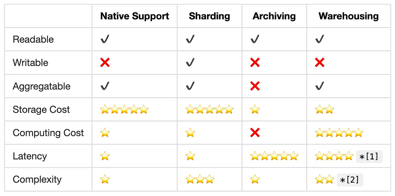
This is exactly strategy 4: data warehousing.

In addition, there are many metadata in the order, and even though we decided to archive order_item, order_payment, and order_delivery, we still want to get the rest of the information in a single query in the data warehouse. Then, we still need to find a way to validate which metadata we want to archive.

At first, we made a few changes to the existing UI to observe user behavior. We want to clarify the following issues.

1. How often users view old data.
2. What kind of old data the user specifically needs.

Our approach is simple: we have added a two-year restriction to the existing time-selection component so that users cannot select a time period longer than two years. Nevertheless, we will not block the user if he queries directly with the order number.

However, we will mask the order details section so that order details older than two years are collapsed based on metadata. When the user clicks on the exact section, we can track which metadata the user really cares about.

Here’s a little trick.

If we collapse all the details, the user’s first reaction will be to click on all of them. Therefore, we opened the basic information of the order, as well as the payment & logistics, and collapsed only those metadata sections that we wanted to validate.

In the end, we verified both the time hypothesis and the user’s need for metadata. Then, we can begin to formally enter the technical selection phase.

Advanced technical selection

Although we chose data warehousing for cold data storage based on the user scenario, there are still many data warehousing options to choose from.

One of the most important considerations is the existing technical stack.

As mentioned in the previous article, if the existing database naturally supports data tiering, then there will not be so many problems. Also, depending on the existing data pipeline in the organization, there may be viable options.

Let’s take a quick look at the SHOPLINE technical stack.

• The (former) main database: MongoDB Atlas
• Main database for data mart: PingCAP TiDB
• Main Warehouse for Data Pipeline: GCP BigQuery

There are three technology options that can be born from these stacks.

Atlas Data Federation

Data federation is a real-time streaming pipeline developed by Atlas that delivers MongoDB data to the object storage system in a near real-time way.

It also builds an API on the object store to provide querying via MQL.

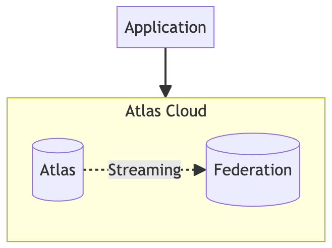
I have to say, this is an excellent solution. Unlike regular data warehouses that offer SQL capabilities, this Atlas self developed data warehouse offers MQL querying capabilities. For an application that is already using MongoDB and MQL, it’s almost a seamless transition.

Furthermore, the data written to this data warehouse can be generated based on specific aggregation statements, making it quicker to satisfy a variety of scenarios.

Nevertheless, Atlas Federation is a technology that can’t be duplicated — after all, it’s Atlas’ own data warehouse. In other words, once we’ve chosen this solution, we’re vendor lock-in.

PingCAP TiDB Serverless

TiDB Serverless is a Compute-Storage Separation architecture, similar to regular data warehouse. It builds a one-tier query engine on top of the object storage system and provides SQL querying capabilities.

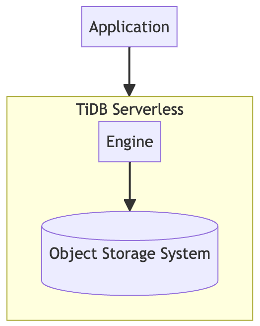
When there are no queries at all, the query engine can be scaled to zero to save costs. In other words, when not in use, TiDB Serverless is only a storage cost. This use case is ideal for cold data storage after data tiering.

For an OLTP database, this would be a brand new invention, but for regular OLAP data warehouse, this is not a big advantage.

For us, if we use this solution, on the one hand, it is another vendor lock-in and on the other hand, we need to rewrite the application program significantly to support SQL query.

If we need to rewrite the application to support SQL, why not use a regular data warehouse such as BigQuery, which we are already using?

GCP BigQuery

I have described our data pipeline in my previous article.

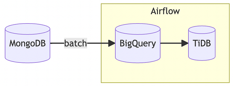
One of the challenges of using BigQuery as a data warehouse for cold data is that BigQuery is not low cost to query. If directly expose BigQuery to the application, then any misuse could be costly, so for the application, we will send the well organized data to the data mart.

If we put all the cold data from all the orders into the data mart, we are creating another object that requires data tiering. But if we don’t use the data mart, then BigQuery would have to be exposed to application queries, which is against our data governance policy.

Second, BigQuery is also a vendor lock-in that we want to get rid of, so we don’t want to add more use cases to BigQuery.

Self-built Data Warehouse

In fact, we have been investigating the option of building our own data warehouse.

The so-called data warehouse is actually a nearly unlimited and low-cost storage space coupled with a scalable computing engine. The lowest entry point is to store Iceberg in AWS S3 and provide query capabilities through Trino.

To investigate the feasibility of Iceberg, I’ve made many attempts to produce several interesting open source playgrounds.

• Integrating Flink with Iceberg
• Integrating Trino with Iceberg

Since it is a practical and feasible approach and is related to our long-term architectural transformation, it will be our answer.

Leverage the existing data pipeline (Fail)

At the beginning, our idea was pretty simple, that is, to leverage the existing data pipeline as much as possible, just put the data into another storage in another format.

So we defined the following architecture.

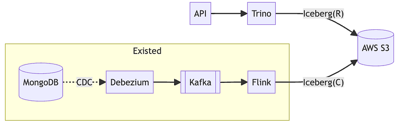
As shown in the diagram, most of our components are ready to go, we just need to establish the ability to read and write to Iceberg, which means we can use a real-time data pipeline to accomplish the conversion from hot data to cold data.

When the life cycle of the data reaches its end, we can delete it in real time, because there is a data pipeline behind it that keeps synchronizing all the data.

The data we want to store is actually what the documents look like in MongoDB, just in Iceberg format in S3.

The following ER model is our data model.

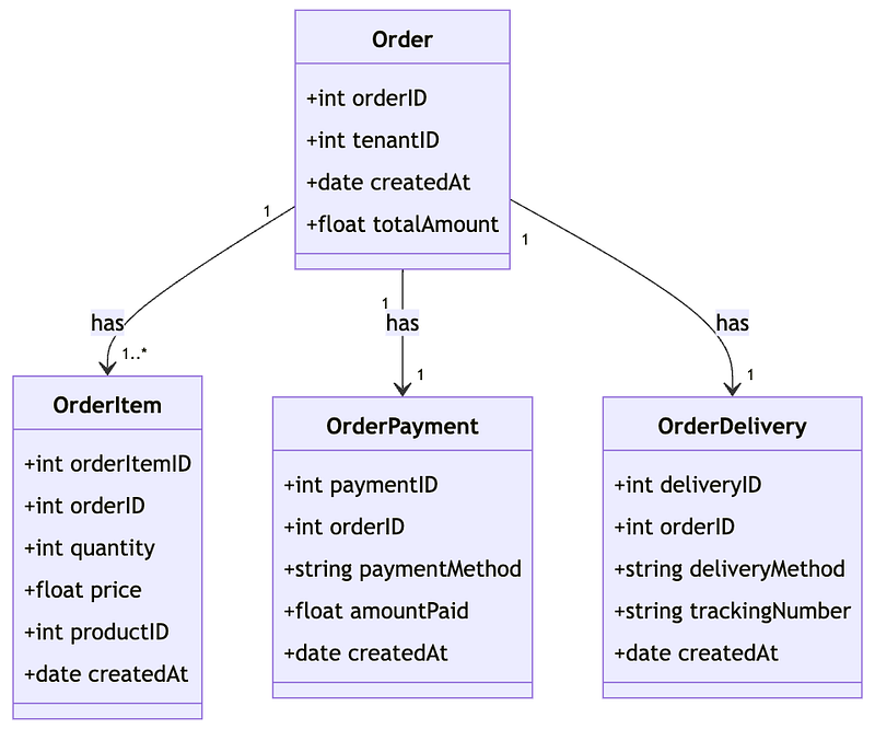
The orderID of the order table is a foreign key to the other metadata tables, so only one SQL command is needed to list the orders in a time period.

SELECT  
    o.orderID,  
    o.tenantID,  
    oi.orderItemID,  
    ...  
FROM  
    order o  
LEFT JOIN  
    order_item oi ON o.orderID = oi.orderID  
LEFT JOIN  
    order_payment op ON o.orderID = op.orderID  
LEFT JOIN  
    order_delivery od ON o.orderID = od.orderID  
WHERE  
    o.orderDate BETWEEN '2024-01-01' AND '2024-01-31'  
ORDER BY  
    o.orderID;

However, we soon realized a problem. It was difficult to choose a common partition key.

The reason why a common partition key is desirable is because we don’t want to couple the data pipeline with the business logic, so each table should be treated in the same way.

Wouldn’t it be better to use orderID? It’s generic and makes business logic.

No, it’s not.

While orderID may seem like the most appropriate option, in Iceberg’s format, the partition key is the core of file granularity, so using orderID as the partition key will result in an endless number of small files scattered across the object store.

This will not only cause inefficiency in querying but also increase the querying cost significantly.

How about using tenantID as the partition key? This is generic enough and makes business logic as well. But as we can see from the ER model above, those metadata tables don’t have tenantID at all.

In that case, we’ll settle for createdAt, which every table has. This may seem like a viable option, but it’s not actually the case. Because the creation date of deliveries, payments, and even order items may not always be the same as the order, this makes it extremely challenging to write a JOIN query using a partition key.

It seems hard to leverage the existing data pipeline and we have to rethink it.

Creating a cold data wide table

Since the original generic ER model is difficult to model in Iceberg, we need to change our implementation.

First of all, we survey all the scenarios where cold data is used, and we realized what we need is to use the order table as the aggregation root, and take out all the related metadata at once. Then it’s easy, we just need to create a wide table.

But who is going to create the wide table?

Not the data pipeline definitely. Because order as the aggregation root has domain logic, if we let the data pipeline build the wide table, then it means the domain logic has to be copied into the data pipeline as well, which greatly increases the coupling of business logic.

Finally, we design a new cold down process.

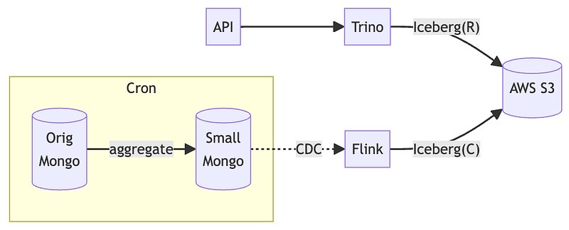
We first set up a tiny MongoDB as a relay to store the wide tables, so that the data pipeline only needs to receive the results of the aggregation. In conclusion, the data pipeline has no business logic at all, and it’s up to the application to decide what data it wants to collect.

The application can delete the processed hot data after the aggregation, and any scenario that requires cold data can be obtained directly through Trino.

Conclusion

In fact, the adoption of self-built data lakehouse for data tiering architecture is our first attempt to transform our data infrastructure.

Architecture transformation is a huge task, through each small task, we can gradually divide and implement the whole big task. In the case of this data tiering, it plays the role of a pioneer, allowing our organization to become familiar with the use of the data lakehouse.

When we have control over the data lakehouse we have built, we have the capital to move on to the next step.

As a result, not only did we reduce the space in our main database by 40%, but we also learned how to implement and maintain a data lakehouse. With this experience, we are now able to face more complex challenges.

Originally published on Medium